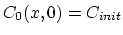
Next: 4 Analytical Solution of
Up: 8 Numerical Handling of
Previous: 2 Discretization of the
3 Discretization of the Three-Stream Mulvaney-Richardson Model
First we consider dopant continuity equation of Mulvaney-Richardson model (3.45).
The local change of dopants is due to the divergence of fluxes of dopant-interstitial and dopand vacancy pairs,
 |
|
|
(154) |
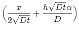
In this model the diffusion coefficient 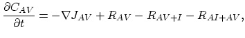 of the point defect-dopant pairs is considered constant and we can write (based on (3.45)),
 ln ln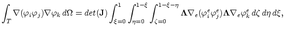 |
(155) |
 ln ln |
(156) |
In order to obtain a weak formulation of (3.92) on the single element
 we multiply both sides of the equation with the basis function
  , and integrate over
  ,
,
 ln ln |
(157) |
 ln ln |
(158) |
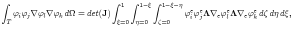
The nonlinear terms of (3.95),
 ,
,
 , and
ln
, and
ln are expressed by the basis nodal functions
 on the following way,
 |
(159) |
 ln ln |
|
In the last expression we used the relationship (3.13) for the electron concentration 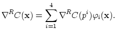 in the case of single charged dopant.
We substitute the relationships (3.96) into (3.95) and obtain,
in the case of single charged dopant.
We substitute the relationships (3.96) into (3.95) and obtain,
 |
|
|
|
 |
|
|
(160) |
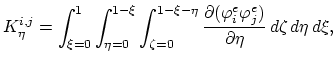
To complete the formulation of the weak equation form we have to evaluate following two integrals,
 |
(161) |
 |
(162) |
here we transfer the calculation to the normed
 coordinate system. Transformation of the gradient operators is done by multiplication with the matrix
 .
.
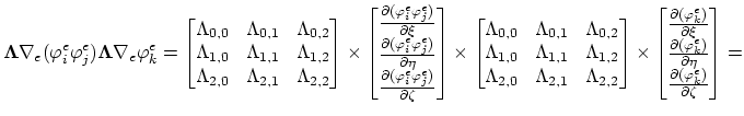
Furthermore we rearrange (3.100),
 |
(164) |
and introduce the matrix
 ,
,
 ,
,
 .
.
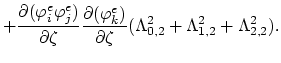
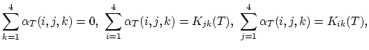
The values of the integrals (3.98) and (3.99) can be expressed as functions of local node indexes,
In (3.103) and (3.104), for the sake of simplicity, we used the abbervations,
 for
for
 .
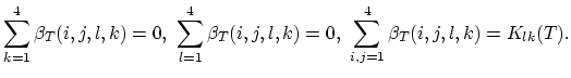
It can easily been shown that the functions
.
It can easily been shown that the functions
 and
and
 satisfy following relations,
 |
|
|
|
 |
|
|
(168) |
We introduce now the backward Euler time discretization scheme for (3.91) and by applying the functions
 and
and
 we write the
 functions (for
  ),
),
 |
(169) |
 |
(170) |
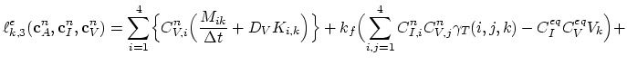
and residuum vector  as
as
 |
|
|
(171) |
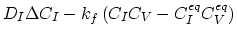
Equations (3.74) and (3.75) of the Mulvaney-Richardson model have the same structure, it is sufficient, if we consider in more detail only (3.74),
 |
|
|
(172) |
We need to consider only
 , the rest of the equation has already been treated above. Again, we use linear basis nodal functions and apply Green's theorem,
 |
|
|
(173) |
we set
 , and proceed,
 |
|
|
(174) |
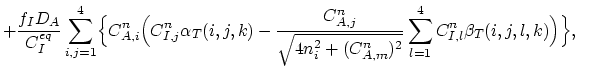
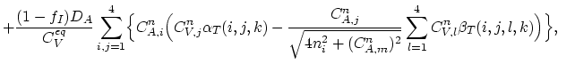
Finally, we have the discretizied form of equation (3.74),
 |
|
|
|
 |
|
|
(175) |
and the residuum vector  as,
as,
 |
|
|
(176) |
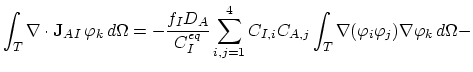
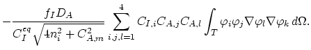
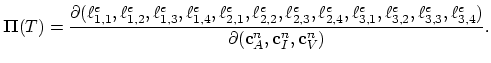
and analogously for the vacancy balance equation,
 |
|
|
|
 |
|
|
(177) |
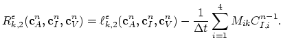
and the corresponding residuum vector  as,
as,
 |
|
|
(178) |
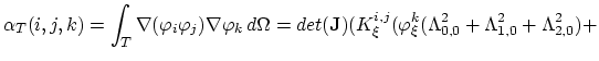
Using the functions
 ,
,
 , and
, and
 for we construct the nucleus matrix
 of the diffusion problem,
 |
(179) |
Note that the global matrix
 in this case has rank
  .
.
Next: 4 Analytical Solution of
Up: 8 Numerical Handling of
Previous: 2 Discretization of the
J. Cervenka: Three-Dimensional Mesh Generation for Device and Process Simulation