Next: 3 Discretization of the
Up: 8 Numerical Handling of
Previous: 1 Discretization of the
2 Discretization of the Simple Extrinsic Diffusion Model
We take the functions
 ,
,
 and
and
 defined on
bounded open domen
defined on
bounded open domen  .
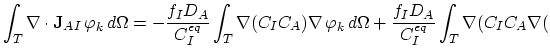
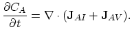
Starting from Green's theorem, a simple relationship can be proved,
.
Starting from Green's theorem, a simple relationship can be proved,
 |
(141) |
where  is the boundary of the domain .
We write (3.33) as
is the boundary of the domain .
We write (3.33) as
 |
(142) |
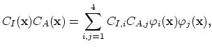
By multiplying (3.79) with the basis function
 and integrating over the domen we have,
 |
(143) |
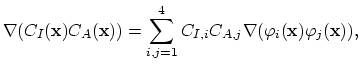
Applying (3.78) on (3.80) gives,
 |
(144) |
Assuming zero-Neumann boundary conditions on we
obtain the weak formulation of the equation (3.33)
 |
(145) |
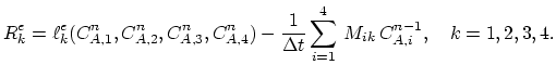
By introducing time discretization with time step 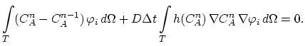 and writing the last equation for the single element
 we obtain,
 |
(146) |
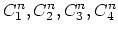
The scalar functions
 ,
,
 , and
, and
 , for
, for
 , are linearly approximated on the element
,
, are linearly approximated on the element
,
The
 , are the values of the concentration at the nodes of the element
  ,
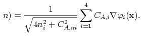
,  is the concentration value at some point inside the .
Normally, for
is the concentration value at some point inside the .
Normally, for
 we use the following simple approximation,
 |
(150) |
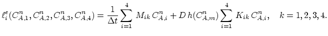
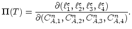
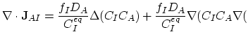
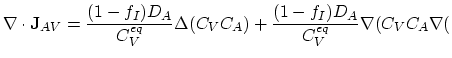
We can define discrete operator  for each
.
Since we have to deal only with a single partial differential equation and not with a system of equations, we can omit the second index in (2.27) by defining the operator,
for each
.
Since we have to deal only with a single partial differential equation and not with a system of equations, we can omit the second index in (2.27) by defining the operator,
 |
(151) |
The nucleus matrix is than defined as
 |
(152) |
and the residuum vector as,
 |
(153) |
The nucleus matrix for this simple case can be also calculated analytically. In this case is also
 .
.
Next: 3 Discretization of the
Up: 8 Numerical Handling of
Previous: 1 Discretization of the
J. Cervenka: Three-Dimensional Mesh Generation for Device and Process Simulation