


Next: 9 Dosis Conservation
Up: 8 Numerical Handling of
Previous: 4 Analytical Solution of
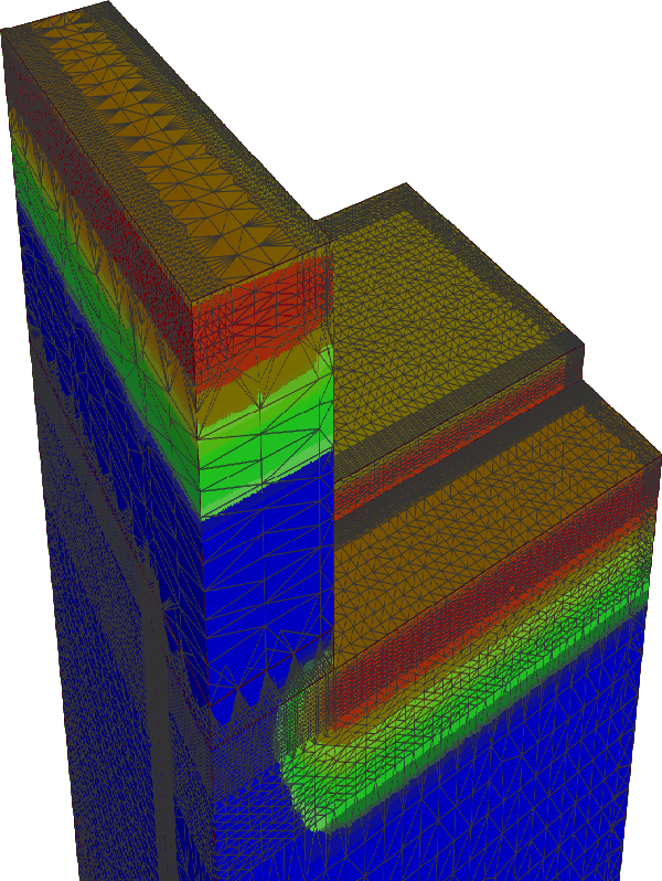
5 Numerical Handling of the Segregation Model
Let us assume that the segments  and
and  are comprised of
three-dimensional areas
are comprised of
three-dimensional areas  and
and  and
the connecting interface
and
the connecting interface  with two-dimensional area
 , respectively. The tetrahedralization of areas ,
and the
triangulation of area are denoted as
, respectively. The tetrahedralization of areas ,
and the
triangulation of area are denoted as
 ,
,
 and
and
 . We discretize (3.30) on the
element
. We discretize (3.30) on the
element
 using a
linear basis function
using a
linear basis function  . After introducing the weak formulation of the equation and subsequently applying Green's theorem we have
 |
(194) |
where  is the boundary of the element
  .
Assuming that
.
Assuming that
 and
marking all inside faces of as
and
marking all inside faces of as
 we have
 and we can write
 |
(195) |
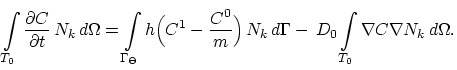
In the standard finite element assembling procedure [5], we take into
account only the terms
 when
building up the stiffness matrix. Thereby the terms
when
building up the stiffness matrix. Thereby the terms
 do not need to be considered because of their annihilation on the inside faces.
The term
 makes sense only on the interface area and
there it can be used to introduce the influence of
the species flux from the neighboring segment area by applying
the segregation flux formula (3.65)
makes sense only on the interface area and
there it can be used to introduce the influence of
the species flux from the neighboring segment area by applying
the segregation flux formula (3.65)
 |
(196) |
After a usual assembling procedure on the tetrahedralization
and
has been carried out and the global
stiffness matrix for both segment areas of the segregation problem has been built,
the interface inputs (3.133) for the segregation fluxes  and
and  are evaluated on the triangulation
and
assembled into the global stiffness matrix according to the particular
assembling algorithm developed in this work.
are evaluated on the triangulation
and
assembled into the global stiffness matrix according to the particular
assembling algorithm developed in this work.
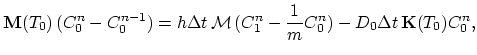
The numerical algorithm based on the concept described above is carried out in two steps.
Step 1.
We assemble the general matrix
 of the
problem for both segments, i.e., for both diffusion processes. The number
of points in segments and is denoted as
of the
problem for both segments, i.e., for both diffusion processes. The number
of points in segments and is denoted as  and
and  ,
respectively. The
general matrix has dimensions
,
respectively. The
general matrix has dimensions
 and the
inputs are correspondingly indexed.
The matrix is assembled by distributing
the inputs from matrix
and the
inputs are correspondingly indexed.
The matrix is assembled by distributing
the inputs from matrix
 ,
,
 , defined for each
 |
(197) |
The 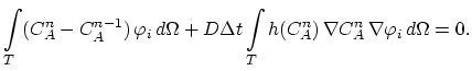 is the time step
of the discretisized time and
is the time step
of the discretisized time and
 and
and
 are stiffness and mass matrix defined on single
tetrahedra
are stiffness and mass matrix defined on single
tetrahedra  from
from

 |
|
|
|
 |
|
|
(198) |
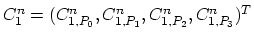
Let us denote vertices of the element
from the tetrahedralization
by
 and their indexes in the segment
  by
by
 . Assembling means, for each
 ,
and
,
and
 adding the term
 to
to
 .
.
After this assembling procedure is carried out the general matrix
has the following structure,
 |
(199) |
Where
 and
and
 . The matrix
 and
and
 are the finite element discretizations of equation (3.30)
for the segments and , respectively.
are the finite element discretizations of equation (3.30)
for the segments and , respectively.
Step 2.
For the element
 with one of it's faces
(
with one of it's faces
(
 ) laying on the interface according to the idea presented above, weak formulation is,
 |
(200) |
The segregation term on the right side of (
 ) is
evaluated on the two-dimensional element
.
If we discretisize equation (
) is
evaluated on the two-dimensional element
.
If we discretisize equation (
 ) and take a backward Euler time scheme with time step , we obtain for segment ,
 |
(201) |
where
 |
(202) |
are the values of the species concentration for the  and
and  time step at the vertices of element
  and analogously
 for
for
 ,
,
 .
Without loosing generality we assume that verticex
.
Without loosing generality we assume that verticex  of the tetrahedras and
  is the point which
doesn't belong to the interface .
In that case the matrix
is the point which
doesn't belong to the interface .
In that case the matrix
 from (
 ) has a simple structure,
 |
(203) |
where
 is the Jacobi matrix evaluated on element
.
Using (3.134) we have,
is the Jacobi matrix evaluated on element
.
Using (3.134) we have,
 |
(204) |
We introduce now
 and
and
 and write for the element ,
 |
(205) |
and analogously for the element ,
 |
(206) |
In the following, for the sake of simplicity, we omit
from
 and write
 .
.
The contributions of
 and
and
 are already included in the
general matrix
by the assembling procedure
made in the first step, the build up of
can now be completed by adding the inputs from matrix
are already included in the
general matrix
by the assembling procedure
made in the first step, the build up of
can now be completed by adding the inputs from matrix
 and
and
 in order to take into account the segregation effect on interface
.
in order to take into account the segregation effect on interface
.
We denote the vertices of the element
 as
as
 . In the tetrahedralization
these points have indices
. In the tetrahedralization
these points have indices
 and indices
 in the tetrahedralization
.
The actual implementation of the scheme (
in the tetrahedralization
.
The actual implementation of the scheme (
 ) is for each
element
of the interface triangulation
and for
:
) is for each
element
of the interface triangulation
and for
:
- adding the term
 to the
input
to the
input

- adding the term
 to the

- adding the term
 to
to
- adding the term
 to the
 .
.
Now the assembling of the general matrix
is
completed. These procedure is carried out for each time step of the simulation.
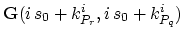
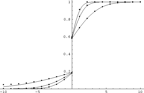
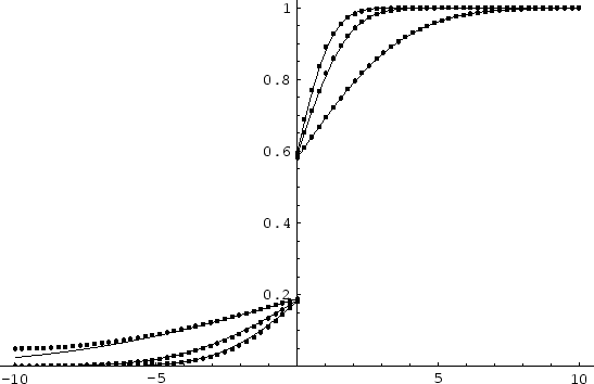
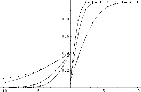
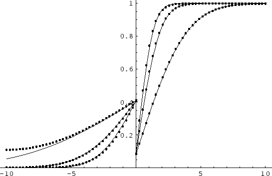
The numerical solution of the segregation problem is compared with an analytical solution on Figure 3.2.
Figure:
The comparison between numerical (points) and analytical
solution (full line) for three different time steps in each figure
above. Two different spatial discretizations (N=20 and N=80 points) are used. Because of
the assumption of the infinite media by the derivation of analytical
solution there is a deviation of this solution from the numerical
one in the proximity of the point  on the abscissa. Numerical solution considers finite segment with zero Neumann boundary condition at the point.
 , , 
|
 , ,
|
|
Next: 9 Dosis Conservation
Up: 8 Numerical Handling of
Previous: 4 Analytical Solution of
J. Cervenka: Three-Dimensional Mesh Generation for Device and Process Simulation