Subsections

• 4.3.1 Black's Law
• 4.3.2 Modeling of the Electromigration Promoting Factors
  • 4.3.2.1 Current density and Joule self-heating
  • 4.3.2.2 Electro-thermal stresses

4.3 Electromigration TCAD Solutions

In order to study electromigration effects in modern copper-based interconnect layouts we have to deal with two types of models which are needed because of the different character of the physical phenomena taking place in the void pre-nucleating and void evolution phase.

We denote as $t_N$ the time needed for the void to nucleate and as $t_E$ the time which a nucleated void needs to grow from some initial nucleation size to the size which changes the interconnect resistivity to such an extent that it practically fails (for example $100\times (R_{actual}/R_{initial}-1)> 20 \%$). So we can calculate the time to failure of the interconnect line,

$$t_f=t_{N}+t_{E}.$$ (4.4)

Until now different TCAD solutions were applied in order to predict the time to failure and possible critical spots of an interconnect structure. The potential critical spots of an interconnect structure are locations where the electromigration promoting factors such as current density, temperature and thermo-mechanical stress reach extraordinary high level.

4.3.1 Black's Law

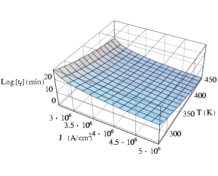
To extrapolate electromigration failure times measured under accelerated test conditions to operating conditions, a semi-empirical model proposed by Black [75] has been widely used in which the time to failure $t_f$ is related to the temperature $T$ and the current density $J$ as

$$t_f = \frac{A}{J^n} (E_a/kT)$$ (4.5)

The current density exponent $n$ and activation energy $E_a$ are determined by experiment. The time to failure distribution according to Black's equation is displayed in Figure 4.1. In addition to this model, Black also observed that using an interconnect metal with a larger grain size leads to increased lifetimes [75].

Figure 4.1: Time to failure as a function of current density and temperature, as predicted by Black's equation.

4.3.2 Modeling of the Electromigration Promoting Factors

4.3.2.1 Current density and Joule self-heating

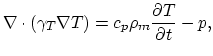
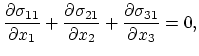
Interconnect reliability due to thermal effects is becoming a serious design issue particularly for dense packed interconnect structures. Thermal effects are inseparable aspects of electrical power distribution and signal transmission through the interconnects due to self-heating caused by the flow of current. Thermal expansion mismatch between the metal and the passivation layer causes stress which leads to fatigue and failure of the metalization [2]. The first problem to be modeled is self-heating due to an electrical current, which is described by the following equations [76],

$$\nabla\cdot(\gamma_T \nabla T)=c_p\rho_m\frac{\partial T}{\partial t}-p,$$ (4.6)

$$p = \gamma_E \Vert\nabla \varphi\Vert^2,$$ (4.7)

$$\nabla\cdot(\gamma_E\nabla\varphi) = 0,$$ (4.8)

where $\gamma_T$ represents the material specific thermal conductivity, $\gamma_E$ is the electrical condutivity, $p$ is the electrical power loss density, $c_p$ is the specific heat, and $\rho_m$ is the mass density. As solution we get the temperature distribution in the interconnect, barrier, and passivation layers.

In each electromigration model discussed below, the effect of electromigration is proportional to current density. Most of the available TCAD electromigration reliability tools [65,68] are exclusively based on current density simulation.

One of the well established results is that the current density exponent $n>1$ in Black's equation is caused by significant Joule self-heating at high current densities [7].

4.3.2.2 Electro-thermal stresses

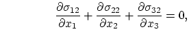
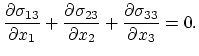
The temperature distribution defined by (4.6)-(4.8) is used to set up the mechanical problem and the required equation for stress development due to thermal expansion is,

$$\sigma_{ij}=B\alpha(T-T_0)\delta_{ij}+\lambda\varepsilon_{kk}\delta_{ij}+2\mu\varepsilon_{ij}.$$ (4.9)

$B$ is the bulk modulus, $\mu$ and $\lambda$ are the Lame' constants, $\alpha$ is the thermal expansion coefficient, and $\varepsilon_{ij}$ are the components of the strain tensor.

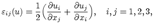
The strain tensor is connected to the local displacements $u_i(x_1,x_2,x_3)$ through relations,

$$\varepsilon_{ij}(u)=\frac{1}{2}\Bigl(\frac{\partial u_i}{\partial x_j}+\frac{\partial u_j}{\partial x_i}\Bigr),\quad i,j=1,2,3,$$ (4.10)

and the mechanical stress equilibrium condition is given by,

$$\frac{\partial \sigma_{11}}{\partial x_1}+\frac{\partial \sigma_{21}}{\partial x_2}+\frac{\partial \sigma_{31}}{\partial x_3}=0,$$

$$\hspace*{1.7cm}\frac{\partial \sigma_{12}}{\partial x_1}+\frac{\partial \sigma_{22}}{\partial x_2}+\frac{\partial \sigma_{32}}{\partial x_3}=0,$$ (4.11)

$$\frac{\partial \sigma_{13}}{\partial x_1}+\frac{\partial \sigma_{23}}{\partial x_2}+\frac{\partial \sigma_{33}}{\partial x_3}=0.$$

Replacing (4.9) and (4.10) into (4.11) one obtains an equation system for unknown local displacement functions $u_i(x_1,x_2,x_3)$.

Equations (4.6)-(4.8) and (4.9)-(4.11) model time dependently the evolution of stress in the interconnect structures. These equations are solved by means of the finite element method [76,11]. After determining local displacement functions $u_i(x_1,x_2,x_3)$, the stress tensor is calculated using relations (4.9) and (4.10).

Depending on the interconnect layout, electro-thermal stresses can have tensile or compressive nature. High tensile stresses can cause break-up of the material and delopement of voids, on the other hand compressive stresses induce generation of extrusions.