


Next: 3 Numerical Implementation
Up: 5 Void evolution and
Previous: 1 Theoretical Formulation
The diffuse interface model equations for the void evolving in an unpassivated
interconnect line are the balance equation for the order parameter  [56,57,58,59],
 |
(260) |
 |
(261) |
and for the electrical field,
 |
(262) |
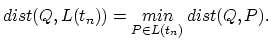
where  is the chemical potential,
 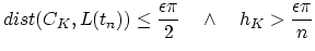 is the double
obstacle potential as defined in [85,86], and
is the double
obstacle potential as defined in [85,86], and  is a parameter controlling the void-metal interface width.
The electrical conductivity was taken to vary linearly from the metal (
is a parameter controlling the void-metal interface width.
The electrical conductivity was taken to vary linearly from the metal (
 ) to the void area (
 ) by setting
 .
The equations (4.50) and (4.52) are solved on the two-dimensional
polygonal interconnect area
.
The equations (4.50) and (4.52) are solved on the two-dimensional
polygonal interconnect area  .
.
It has been proven [57,59] that in the asymptotic limit for
 the diffuse interface model defined by equations
(4.50)-(4.52) describes the same voids-metal interface
behavior like equations (4.43)-(4.48). The width of the
void-metal diffuse interface is approximately
the diffuse interface model defined by equations
(4.50)-(4.52) describes the same voids-metal interface
behavior like equations (4.43)-(4.48). The width of the
void-metal diffuse interface is approximately
 , and in
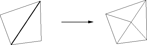
order to numerically handle sufficiently thin interfaces one needs a very fine
locally placed grid around it.
, and in
order to numerically handle sufficiently thin interfaces one needs a very fine
locally placed grid around it.
Next: 3 Numerical Implementation
Up: 5 Void evolution and
Previous: 1 Theoretical Formulation
J. Cervenka: Three-Dimensional Mesh Generation for Device and Process Simulation