3.4 Dislocation in an anisotropic continuum
Steeds [72] developed a treatment to derive the dislocation energy within the
anisotropic elasticity. According to this treatment, the dislocation is considered
straight and extended to infinity along the z-axis. This assumption simplifies the
problem to a plane strain problem where no quantity depends on the z-coordinate,
so
 | (3.17) |
The Burgers vector of the dislocation is b. Displacements are given by the functions ux, uy
and uz. The displacements ux and uy correspond to the edge component of the considered
dislocation whereas uz corresponds to the screw component. The strain components
are
| εxx =  ,εxz = ,εxz =   , , | |
|
| εzz = 0,εxy =  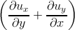 , , | (3.18)
|
| εyy =  ,εyz = ,εyz =   . . | | |
The previous equations relate the six strain components to the three components of the
lattice displacement and this implies that relations exist between the various εij. These
relations are known as the compatibility equations [45]:
|  + +  = 2 = 2 , , | (3.19a)
|
|  - - = 0. = 0. | (3.19b) |
Hooke’s law for an anisotropic material is written as:
 | (3.20) |
The infinite straight dislocation lies along the z-axis and therefore εzz = 0. This last relation
yields an additional condition:
| 0 = εzz = s21σxx + s22σzz + s23σyy + s24σyz + s25σxy + s26σxz, | |
|
| σzz =  ∕s22. ∕s22. | (3.21) |
Steeds [72] expressed the stresses as a function of the Airy functions, F and ϕ
| σxx =  ,σxz = - ,σxz = - , , | |
|
| σxy = - ,σyz = - ,σyz = - , , | |
|
| σyy =  . . | (3.22) |
Substituting the expressions (3.21) and (3.22) into the compatibility equations (3.19)
yields
|   + s12 + s12 + s21 + s21 + + | |
|
|   + + | |
|
| s66 + s15 + s15 + s25 + s25 + s64 + s64 = = | |
|
|   | |
|
|   + + | |
|
| s16 + s26 + s26 + s61 + s61 + s62 + s62 + + | |
|
| s14 + s24 + s24 + s65 + s65 , , | (3.23a)
|
| |
|
| s11 + s12 + s12 + s21 + s21 + s22 + s22 + + | |
|
|   + + | |
|
| s66 + s15 + s15 + s25 + s25 + s64 + s64 = = | |
|
|   + + | |
|
| s16 + +   + + | |
|
| s26 + s61 + s61 + s62 + s62 + s14 + s14 + s24 + s24 + s65 + s65 . . | (3.23b) |
Solutions for the previous equations with cylindrical symmetry have the following
form [72]:
F = Bg ,ϕ = Cf ,ϕ = Cf , , | | (3.24) |
where g and f are functions of a linear combination of the coordinates x and y.
Substituting (3.24) into (3.23) and eliminating B and C yields a sextic equation for the
parameter p:
| p6 - - | |
|
| 2p5 + + | |
|
| p4 - - | |
|
| 2p3 + + | |
|
| p2 - - | |
|
| 2p + + | |
|
| S22S44 - S242 = 0 | (3.25) |
where Slm = slm - . Roots of this equation occur as pairs of complex
conjugates p1 and p1*, p
2 and p2*, and p
3 and p3*. Therefore the most general solution for
the functions F and ϕ are
. Roots of this equation occur as pairs of complex
conjugates p1 and p1*, p
2 and p2*, and p
3 and p3*. Therefore the most general solution for
the functions F and ϕ are
F = ∑
n=13 , , | | (3.26a)
|
ϕ = ∑
n=13 , , | | (3.26b) |
where n = 1, 2, 3, ζn = x + pny, and gn and fn denote, respectively, the functions g and f
belonging to the root pn. In order to satisfy the physical expectations that the stress field
decays as 1/r, it is required that
Substituting (3.26) and (3.27) into (3.22) causes the stress components to become
| σxx = ∑
n=13 , , | |
|
| σxy = -∑
n=13 , , | |
|
| σyy = ∑
n=13 , , | |
|
| σxz = ∑
n=13 , , | |
|
| σyz = -∑
n=13 , , | (3.28) |
The displacement components are obtained combining (3.18) and (3.26):
| ux = | ∫
εxxdx = | |
|
| ∑
n=13 | ![{[( ) ]
S11p2n - S16pn + S12 Bn + (S15pn - S14)Cn lnζn](DISS187x.png) | |
|
| ![[( *2 * ) * * *] *}
S11p n - S16pn + S12 Bn + (S15pn - S14)C n ln ζn](DISS188x.png) , , | (3.29a)
|
| |
|
| uy = | ∫
εyydz = | |
|
| ∑
n=13 | ![{[( ) ]
S12p2n - S26pn + S22 Bn + (S25pn - S24)Cn lnζn](DISS189x.png) | |
|
| ![[( *2 * ) * * *] *}
S12p n - S26pn + S22 Bn + (S25pn - S24)C n ln ζn](DISS190x.png) , , | (3.29b)
|
| |
|
| uz = | ∫
εxzdx = | |
|
| ∑
n=13 | ![{[( ) ]
S15p2 - S56pn + S25 Bn + (S55pn - S45)Cn lnζn
n](DISS191x.png) | |
|
|  . . | (3.29c)
|
| | |
In order to evaluate the quantities Bn and Cn and their complex conjugates, six
relationships are required.
The first set of boundary conditions is derived from the force equilibrium state of the
media, i.e., the condition of zero net force on the dislocation [72], expressed
as
 S ∑
jσijnjdS = 0, S ∑
jσijnjdS = 0, | | (3.30) |
for an arbitrary cylindrical surface S enclosing the dislocation line. nj denotes components
of the outer normal to the integration surface S. For an infinite straight dislocation along
the z-axis, the previous equation becomes
 S ∑
jσijnjdS = 0, S ∑
jσijnjdS = 0,  . . | | (3.31) |
It is assumed that the cylinder S has a height  with a circular base
  on the xy-plane.
Based on these assumptions, the previous equation yields for i = x
on the xy-plane.
Based on these assumptions, the previous equation yields for i = x
0 =  S S dS = ∫
Cd dS = ∫
Cd = = ![[ ]
∂F
----
∂y](DISS199x.png) , , | | (3.32) |
and when substituting the expression for F from (3.26) and using (3.27) one
gets [72]
![[ ]
∑3 * * *
(Bnpn ln ζn + Bnp nlnζn)
n=1](DISS200x.png)  = 0. = 0. | | (3.33) |
The start and the end point of the closed integration loop differ by the argument
Δθn = 2π. Since the logarithm of a complex argument can be written as
| ln ζn = ln rn + iθn, | | (3.34a)
|
| ln ζn* = ln r
n*- iθ
n, | | (3.34b) |
equation (3.33) becomes
∑
n=13![[Bnpn (lnrn + i2π - lnr ) + B *np*n (ln r*n - i2π - ln r*n)]](DISS201x.png) = 0. = 0. | | (3.35) |
Simplifying, one gets
∑
n=13 = 0. = 0. | | (3.36) |
Analogously, another two conditions are obtained from equation (3.33) for i = y
∑
n=13 = 0, = 0, | | (3.37) |
and for i = z
∑
n=13 = 0. = 0. | | (3.38) |
The second set of boundary equations is provided by the displacement relations. The
integral of the displacement acquisitions along the Burgers circuit encircling the dislocation
line must be equal to the Burgers vector b:
Substituting equations (3.29) for the displacements components into the last relation yields
a set of three equations of the form bi∕2πi = QniBn - Qni*B
n*. More explicitly the last
three equations become
| bx = | 2πi∑
n=13![[ ( 2 * *2) * * ]
S11 Bnp n - B npn + S15 (Cnpn - C npn)](DISS205x.png) , , | (3.40a)
|
| by = | 2πi∑
n=13 | |
|
| ![+ (S + S )(C p - C *p*) - S (C p2 - C *p*2)]
56 14 n n n n 15 n n n n](DISS207x.png) , , | (3.40b)
|
| bz = | 2πi∑
n=13![[ ( ) ]
S15 Bnp2n - B *np*n2 + S55 (Cnpn - C *np*n)](DISS208x.png) . . | (3.40c) |
The stress field of the dislocation is fully described by equations (3.28) where constants
pn are the roots of equation (3.25) and constants Bn are the solution of the system of linear
equations (3.36), (3.37), (3.38) and (3.40).
The calculation of the dislocation energy is performed by substituting the stress
components in equation (3.15) along the cut surface described by the coordinate r such that
x = r sin φ and y = r cos φ. The components of the outer normal n are nx = cos φ, nz = 0
and ny = sin φ. The inner and outer cut-off radii are rc and R, respectively. Then one
obtains
 | =  ∫
rcR ∑
n=13 ∫
rcR ∑
n=13 | |
|
| + ![]
(bxB*np*n-+-byC-*n --bzB*n)-p*nsinφ-+--(--bxB-*np*n---byCn*+-bzB-*n)cosφ--
cosφ + p* sin φ
n](DISS212x.png)  = = | |
|
| =  ∑
n=13 ∑
n=13![[Bn (- bxpn + bz) - Cnby + B * (- bxp* + bz) - C*by]
n n n](DISS215x.png) ln ln  = = | |
|
| = K ln  , , | (3.41) |
where K is the so called pre-logarithmic coefficient of the dislocation energy. K depends on
the elastic constants, the Burgers vector b and the particular direction of the dislocation
line with respect to the crystallographic axes.
 =
=  =
=  .
.