Appendix B

From (4.118) and (4.119) we get

$$a_{44} = \frac{\Omega_{100}-\Omega_{110}}{210}$$ (6.10)

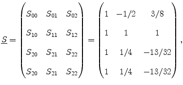
After elimination of $a_{44}$, the system of equations (4.118) to (4.122) can be expressed in matrix form as

$$\ensuremath{{\underline{S}}}\cdot \ensuremath{{\underline{Z}}} = \ensuremath{{\underline{B}}}$$ (6.11)

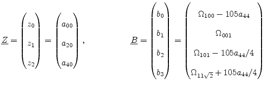
where

$$\ensuremath{{\underline{S}}} = \begin{pmatrix}S_{00} & S_{01} & S... ... -1/2 & 3/8 1 & 1 & 1 1 & 1/4 & -13/32 1 & 1/4 & -13/32 \end{pmatrix},$$ (6.12)

$$\ensuremath{{\underline{Z}}} = \begin{pmatrix}z_{0} z_{1} z_... ... \Omega_{101} - 105a_{44}/4 \Omega_{11\sqrt{2}} + 105a_{44}/4 \end{pmatrix}$$ (6.13)

To determine the four coefficients from the overdetermined system (6.11), we solve (4.118) to (4.120) exactly and minimize the error in  (4.121) and (4.122). Since $S_{00} = S_{10} = S_{11} = S_{12} = S_{20} = 1$, using the new variables the equations can be written as

$$z_0 + S_{01}z_1 + S_{02}z_2 - b_0 = 0,$$ (6.14)

$$z_0 + z_1 + z_2 - b_1 = 0,$$ (6.15)

$$z_0 + S_{21}z_1 + S_{22}z_2 - b_2 \rightarrow \ensuremath{{\mathrm{Min}}},$$ (6.16)

$$z_0 + S_{21}z_1 + S_{22}z_2 - b_3 \rightarrow \ensuremath{{\mathrm{Min}}}.$$ (6.17)

Next, we eliminate $z_0$ by subtracting (6.15) from (6.14), (6.16), and (6.17).

$$(S_{01} - 1)z_1 + (S_{02} - 1)z_2 + b_1 - b_0 = 0$$ (6.18)

$$(S_{21} - 1)z_1 + (S_{22} - 1)z_2 + b_1 - b_2 \rightarrow \ensuremath{{\mathrm{Min}}}$$ (6.19)

$$(S_{21} - 1)z_1 + (S_{22} - 1)z_2 + b_1 - b_3 \rightarrow \ensuremath{{\mathrm{Min}}}$$ (6.20)

To eliminate $z_1$, (6.18) is multiplied by $\tau = (S_{21}-1)/(S_{01}-1)$ to obtain

$$(S_{21} - 1) z_1 + \tau (S_{02} - 1) z_2 + \tau (b_1 - b_0) =0.$$ (6.21)

Subtracting (6.21) from (6.19) and (6.20) gives

$$f_1 = uz_2 + v \rightarrow \ensuremath{{\mathrm{Min}}},$$ (6.22)

$$f_2 = uz_2 + w \rightarrow \ensuremath{{\mathrm{Min}}},$$ (6.23)

with

$$u = (S_{22}-1) - \tau (S_{02}-1),$$ (6.24)

$$v = b_1 - b_2 - \tau (b_1-b_0),$$ (6.25)

$$w = b_1 - b_3 - \tau (b_1-b_3).$$ (6.26)

The least square minimum can be obtained by setting the derivative to zero,

$$\frac{\partial f_1^2}{\partial z_2} + \frac{\partial f_2^2}{\partial z_2} = 2 (uz_2 +v) u + 2 (uz_2 + w) u = 0,$$ (6.27)

which gives

$$z_2 = -\frac{v +w}{2u}.$$ (6.28)

With the definitions (6.24) to (6.26) and using (6.12) we get

$$z_2 = -\frac{16}{35} (-b_0 - b_1 + b_2 + b_3),$$ (6.29)

$$z_1 = \frac{2}{3} (b_0 + b_1) - \frac{5}{12}z_2,$$ (6.30)

$$z_0 = \frac{2}{3} (-b_0 + b_1/2) - \frac{7}{12}z_2.$$ (6.31)

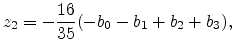
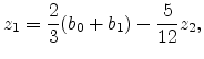
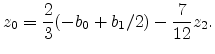
Substituting back the value of $b_i$'s from (6.13) into (6.29) to (6.31) gives equations (4.123)-(4.126).