6.2.1 Discretization

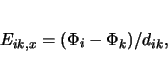
For the box integration method a flux vector has to be calculated at each box boundary. MINIMOS-NT offers an elegant approach where the vector quantities only have to be stored at the grid points and the resulting quantities at the boundaries are reconstructed [Fis94]. The electric field $E_{ik}$, e.g., which occurs at the boundary between the boxes i and k, is calculated using the following algorithm: The component perpendicular to the boundary $E_{ik,x}$ is calculated as the gradient of the potentials $\Phi_i$ and $\Phi_k$,

$$E_{ik,x}=(\Phi_i-\Phi_k)/d_{ik},$$ (6.3)

where $d_{ik}$ is the distance between the two grid points. The parallel component $E_{ik,y}$ is calculated in two steps. First, the electric fields $\vec{E}_i$ and $\vec{E}_k$, which occur at the grid points, are calculated by a second order Taylor expansion with the potentials of all the neighboring gridpoints and the gridpoint itself as arguments [Fis94].

In order to get the correct representation at the boundary, a linear extrapolation between the parallel components of the neighboring electric fields $\vec{E}_i$ and $\vec{E}_k$ is performed,

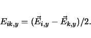$$E_{ik,y}=(\vec{E}_{i,y}-\vec{E}_{k,y})/2.$$ (6.4)