Validation

4.4 Validation

The improvements which have been made to the algorithms of the signed-particle method, presented in this chapter, have increased the accuracy of WMC simulations. To illustrate this fact (and for validation purposes) a comparison is made here between the exact solution of the time-dependent Schrödinger equation and results obtained by the WMC method.

A general, exact solution of the time-dependent Schrödinger equation can be calculated by

∫ ψ (x,t) = dx′K (x,t;x′,t0)ψ (x′,t0) , (4.18)

where K

is the propagator function associated to the stationary Hamiltonian describing the system and ψ (⋅,t)
0

is the initial condition of the wave function.

As a benchmark problem a wavepacket travelling towards a square potential barrier, to its right, within a closed system is considered here. The minimum uncertainty wavepacket, which serves as an initial condition, is defined as

( 2)- 1∕4 - (x-x0)22 ik0z ψ (x,t0) = 2πσ e 4σ e , (4.19)

with parameters given in Table 4.5. The potential considered here (square barrier) gives rise to analytic expressions for the propagator [142], allowing an exact solution of the Schrödinger equation to be obtained by a numerical integration of (4.18). This exact solution avoids approximations associated to numerical treatments and serves as a reliable basis for validation of the results obtained by the WMC simulator.

Table 4.5: Simulation parameters for validation example

x₀ [nm]	σ [nm]	L_coh [nm]	k₀ [nm^-1]	Δx [nm]
-29.5	10	100	12Δk	0.1

Figure 4.18: Charge density at various time steps for a wavepacket (mean energy of 0.067eV) approaching a 4nm wide, 0.1eV high barrier.

Figure 4.19: The k-distributions, corresponding to Figure 4.18, at 0fs and 100fs showing the reflection and transmission from/through the barrier of a wavepacket initially centred around 12Δk.

Figure 4.20: Charge density at various time steps for a wavepacket (mean energy of 0.067eV) approaching a 4nm wide, 0.3eV high barrier.

Figure 4.21: The k-distributions, corresponding to Figure 4.20, at 0fs and 100fs, showing almost complete reflection from the barrier.

The Wigner transform is applied to (4.19) to obtain the corresponding Wigner function, which serves as an initial condition for the WMC simulation:

1 - (x-x0)2 -(mΔk- k0)22σ2 f (x,m, t0) = π-e 2σ2 e . (4.20)

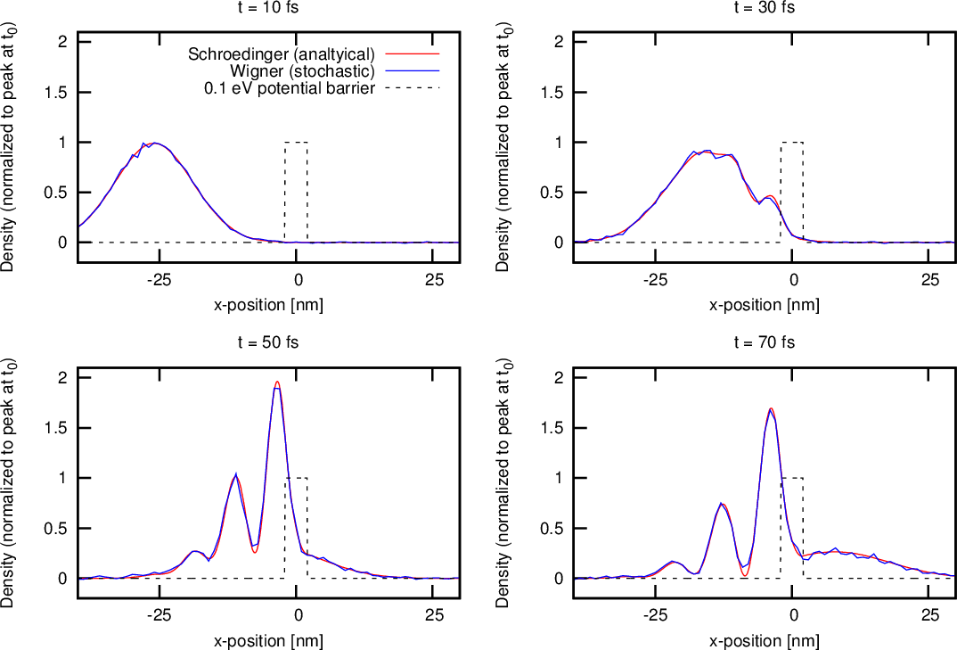
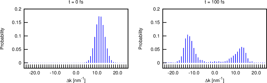
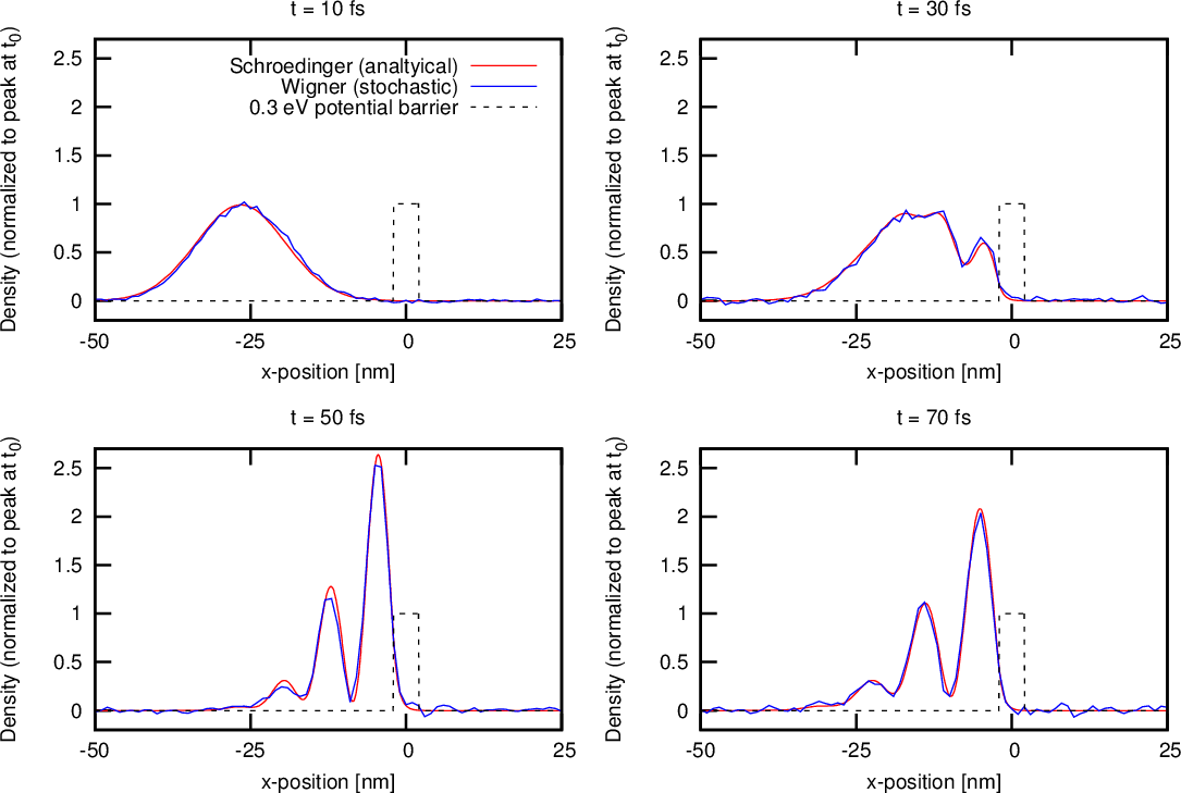
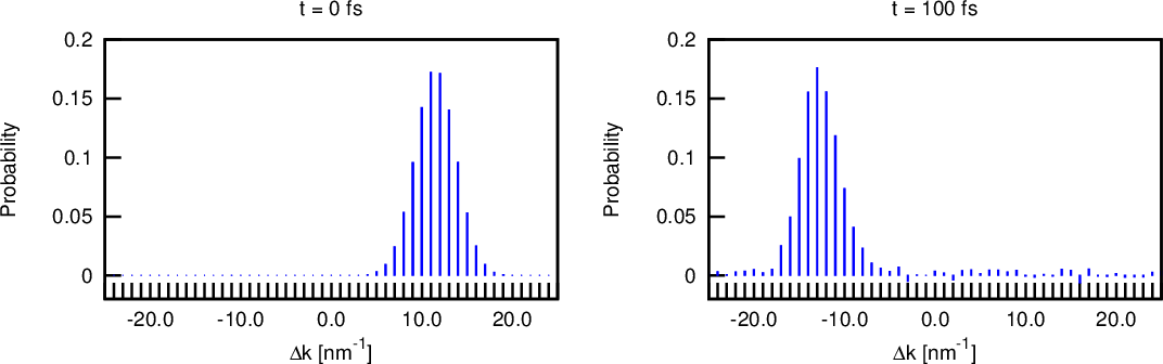
Figure 4.18 compares the solution obtained by the WMC method and the exact solution of the corresponding Schrödinger equation, over a time sequence, for a 4nm wide, 0.1eV barrier – the mean energy of the wave package is 0.067eV. The transmitted and reflected components of the wavepacket are evident, as supported by the k-distributions in Figure 4.19. Previous comparisons between results obtained by the Schrödinger equation and Wigner Monte Carlo simulations have failed to show a truly quantitative match [143]. Here, an excellent match between the stochastic solution of the Wigner equation and an exact solution of the Schrödinger equation is evident (as was first reported in [144]) thanks to the optimized algorithms and considerations presented in this chapter. The Monte Carlo solution shows some noise, due to the stochastic nature of the method, especially the particle generation process.

Figure 4.20 and Figure 4.21 show the result of the same wave package approaching a 0.3eV barrier, which leads to almost complete reflection. The simulation required a fine spatial resolution (0.1nm) to appropriately represent the sharp edges of the square barrier along with an appropriately chosen coherence length (cf. Table 4.5).

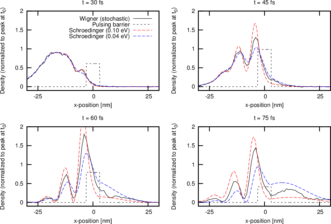
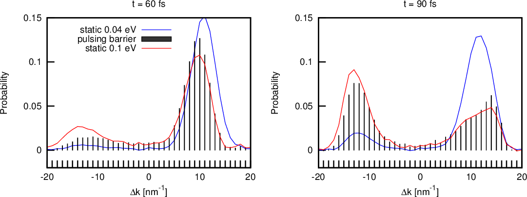
Unlike for the discussed analytical method, the ability to include an arbitrary, time-dependent potential in the WMC simulator is a big advantage. This, however, requires the WP, V _w, to be recomputed at each time step. The computational cost of the latter can be high (especially in higher dimensions), but can be significantly reduced by using the specialised, box discrete Fourier transform (discussed in Section 4.1.2), which exploits the correlation between the values of V _w amongst adjacent nodes. As a validation of the WMC results, incorporating a time-dependent potential, the potential barrier is made to rapidly oscillate between 0.04eV and 0.1eV with a period of 20fs, and the result is compared to the bounds set by the exact solutions of the limiting (static) cases in the spatial domain, as illustrated in Figure 4.22. Figure 4.23 shows the k-distributions of the stochastic solutions for the dynamic potential and the two limiting, static potentials – the solution for the oscillating barrier remains within the set static bounds. Moreover, a reflection of the wavepacket (0.067eV) against the static 0.04eV barrier can be identified, which is consistent with the expected quantum behaviour.

The increased accuracy is attributed primarily to improved generation statistics (Section 4.2) and the use of a sufficient wavevector resolution (through the choice of the coherence length). The increase in the computational demands of a large coherence length can be significant in 2D simulations but can be alleviated by the algorithms presented in Sections 4.3 and 4.1.2.

The presented benchmark tests show that the WMC method has been matured to the point of providing highly accurate results, thanks to appropriate handling of the particle-generation statistics (Section 4.2) and the appropriate choice for the mesh resolution. The presented considerations conceptually extend to higher dimensions, thereby paving the way for the accurate numerical analysis of mesoscopic semiconductor devices using the Wigner formalism.

Figure 4.22: Charge density at various time steps for a 6nm wide barrier oscillating between 0.04eV and 0.1eV. The simulated solution (Wigner) with a dynamic potential remains between the bounds given by exact solutions of the Schrödinger equation for the static, limiting cases.

Figure 4.23: Comparison of the k-distributions (obtained by WMC) of the pulsating barrier and the static barriers of the limiting cases, as in Figure 4.22.

[prev] [prev-tail] [front] [up]