 (b)
(b)
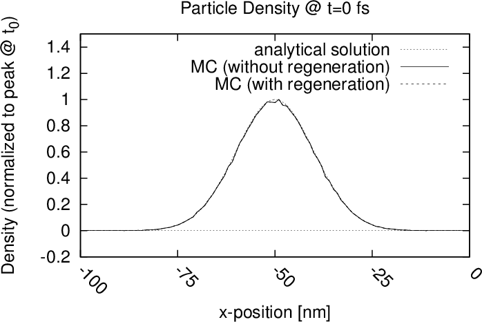
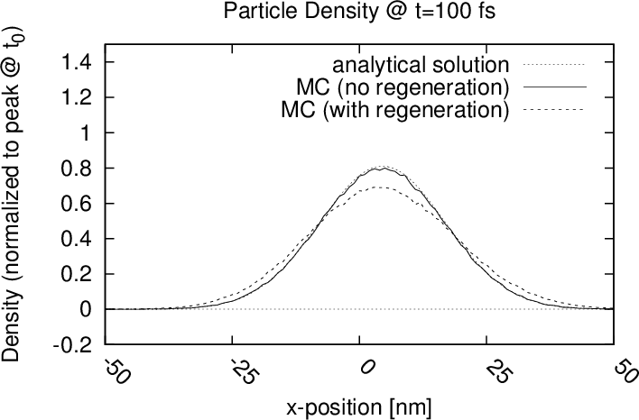
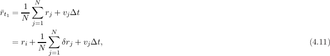
Figure 4.12: Comparison of a wavepacket evolved from (a) 0fs to (b)100fs, using an analytical solution and a Monte Carlo (MC) approach without and
with the regeneration process (repeated every 0.1fs).
The concept of particle annihilation has been introduced in Section 3.7.6. The annihilation procedure is the crucial aspect of the signed-particle method, which has made multi-dimensional simulations computationally feasible. For this reason the effects of the approximations that are made are given careful consideration in this section. Moreover, two alternative implementations of the annihilation algorithm are presented, which reduce or completely eliminate the huge memory demands of the conventional annihilation algorithm.
The phenomena of numerical diffusion brought about by the regeneration of particles has been identified in [139] and is reviewed in the following.
(b)
After the annihilation of particles within a cell has taken place, the remaining particles have to be regenerated. The conventional approach to selecting the position of the regenerated particles is to spread the particles uniformly across the cell. This approach, however, may lead to a ’numerical diffusion’ of particles, which causes the global particle ensemble to propagate at a different rate than dictated by its k-distribution. To demonstrate this numerical artefact the following example is considered.
A 1D minimum uncertainty wavepacket of the form (3.34) with ro = -50nm, k0 = 6 nm-1 and σ = 10nm propagates in a domain with zero potential. The
evolution of the wavepacket is compared in Figure 4.12 using three different approaches: i) an analytical solution, ii) a Monte Carlo approach
without any regeneration and iii) a Monte Carlo approach with a (forced) regeneration procedure at each time step (a typical value for the
annihilation of 0.1fs is chosen). It is evident that the approaches i) and ii) correspond exactly, however, the wavepacket which is subjected
to the regeneration procedure spreads out faster. This discrepancy must be attributed to the regeneration procedure and is analysed in the
following.
nm-1 and σ = 10nm propagates in a domain with zero potential. The
evolution of the wavepacket is compared in Figure 4.12 using three different approaches: i) an analytical solution, ii) a Monte Carlo approach
without any regeneration and iii) a Monte Carlo approach with a (forced) regeneration procedure at each time step (a typical value for the
annihilation of 0.1fs is chosen). It is evident that the approaches i) and ii) correspond exactly, however, the wavepacket which is subjected
to the regeneration procedure spreads out faster. This discrepancy must be attributed to the regeneration procedure and is analysed in the
following.
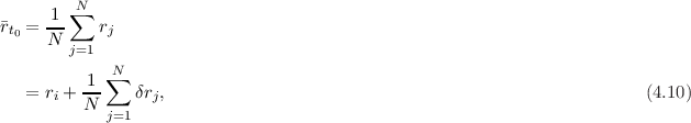
Consider an ensemble of N particles, with positions  j = 1…N,rj ∈Ωi, within the cell (i,q) at time t0. The mean position of the ensemble at time t0
is
j = 1…N,rj ∈Ωi, within the cell (i,q) at time t0. The mean position of the ensemble at time t0
is
 j = 1…N′≤ N. If the particles are uniformly distributed over the cell, one imposes
The original spatial distribution of the particles within a cell can be perfectly recovered, if all (infinitely many) of the moments of the distribution before the annihilation are known (and the Carleman’s condition for uniqueness is satisfied [140]). The mean position represents the first moment of the local distribution and already retains the most important information. By uniformly distributing the particles over a distance Δr around the pre-annihilation mean, the ’numerical diffusion’ is effectively remedied, albeit with some added ’noise’, as shown in Figure 4.13. This ’noise’ is attributed to the fact that the uniform distributions of neighbouring cells overlap.
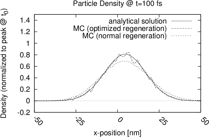
If, in addition to the mean, the second moment of the distribution – the standard deviation – is also calculated the particles can be regenerated using e.g. a Gaussian distribution. The result, shown in Figure 4.14, is very noisy, however, since a Gaussian distribution poorly models the actual distribution in each cell: the Gaussian distribution approaches zero in both directions, whereas the actual particle distribution has a non-zero value at the boundaries of the cell. All the common statistical distributions (Gaussian, exponential, beta etc.) tend towards zero on at least one tail, which makes them unsuitable to obtain a satisfactory fit with the particle distribution in a single cell.
In summary, an artificial propagation/retardation of particles (’numerical diffusion’) arises, when the spatial distribution of particles, within a phase-space cell, is not considered prior to the annihilation for the subsequent regeneration. By calculating the mean position of the particles in a cell before annihilation takes place presents an effective way to avoid this ’numerical diffusion’. The computational costs of this approach remains almost negligible (<1% for the presented cases) and, therefore, is well-suited for problems where computational penalty of simply decreasing Δr would be intolerable. The proposed solution presents another optimization which makes the WMC simulations more computationally efficient and thereby more accessible for users with limited computational resources.
The memory required to represent the phase space grid, on which particles are recorded for annihilation, quickly becomes exorbitant in multi-dimensional simulations with a fine spatial resolution, since the number of cells increases with the power of the dimensionality of the phase space (the resolution also affects the number of k-values which must be retained to ensure a unitary Fourier transform). A high spatial resolution is required is required to investigate certain problems, e.g. the direct modelling of surface roughness discussed in Appendix C.
 (b)
(b)
A 30nm × 30nm domain and a three-dimensional k-space with a coherence length of 30nm results in an array size exceeding 141GB at a resolution of 0.2nm. Chapter 5 presents a distributed-memory (MPI) parallelization approach to address these large memory requirements, using a spatial domain decomposition. However, the computational demands of the signed-particle WMC simulator allow it to be run on a typical desktop computer, therefore, its memory demands should also follow suit.
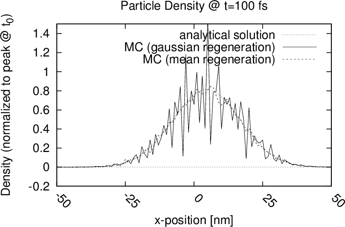
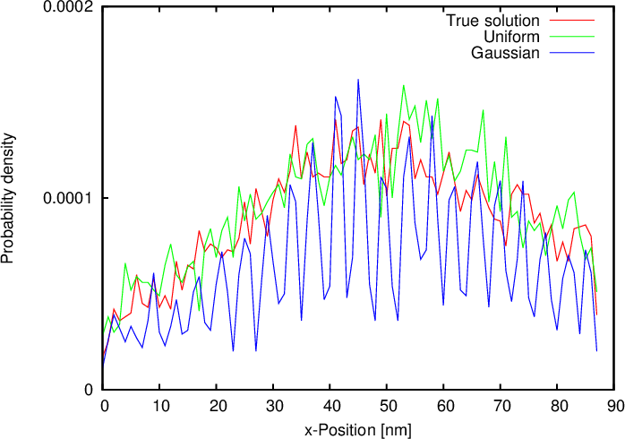
A possibility to reduce the memory requirements of the annihilation algorithm is to reduce the spatial resolution of the grid on which the particles are recorded for annihilation; the resolution of the k-values and the potential mesh remain unaltered. The concept is depicted in Figure 4.15. To counteract the loss in resolution, the spatial distribution of the particles in the enlarged cell is fitted to a statistical distribution before annihilation ensues. The obtained distribution is then used to regenerate the particles which remain after the annihilation – essentially, the approach presented in Section 4.3.1 to counteract numerical diffusion is applied here for a bigger spatial area to reduce the memory requirements.
Figure 4.16 compares the regeneration of particles, annihilated on a coarsened grid, using a uniform distribution and a Gaussian distribution around the pre-annihilation mean position of particles. The former follows the true solution much better than the Gaussian distribution which provides a poor approximation of the distribution in each cell; this is consistent with the observations made in the preceding section. The use of a Gaussian distribution artificially re-introduces information which conflicts with the assumption made to perform annihilation, namely that all particles in a cell are considered to be indistinguishable regardless of their position. The uniform distribution best reflects this state of information.
Regenerating particles over an area corresponding to one annihilation cell, centred on the mean position of all particles (both positive and negative) before the annihilation, is justified by the observation that the area of the cell that is highly populated has better statistics (lower variance). Therefore, the variance is minimized in some sense by generating particles across the area of a cell centred at the pre-annihilation mean, instead of uniformly across the cell (i.e. a mean forced to be at the centre of the cell).
In summary, a reduction of the spatial resolution of the phase space grid used for annihilation reduces the memory requirements. By fitting the pre-annihilation spatial distribution of particles in a cell to a statistical distribution, the loss in resolution can be mitigated. Under the assumptions made for annihilation the uniform distribution is best-suited; other common statistical distributions, like Gaussian distributions, are ill-suited for the fitting and require some extra memory and computation to calculate the additional moment of the distribution (the standard deviation).
The representation of the phase-space as an array to record the signs of particles is a direct reflection of the physical concept underlying particle annihilation. However, the annihilation concept can be also realized with an algorithm which avoids representing the phase space by an array, thereby completely avoiding the huge memory demands associated with it. This novel algorithm presents a significant contribution to making WMC simulations computationally more accessible and is presented in the following.
An integer index can be associated to the position and momentum attributed to each particle. These indices are mapped to a single integer H, uniquely identifying the cell of the phase space in which the particle resides:


 time complexity. As N can be several millions, the additional
computation time is not tolerable.
time complexity. As N can be several millions, the additional
computation time is not tolerable.
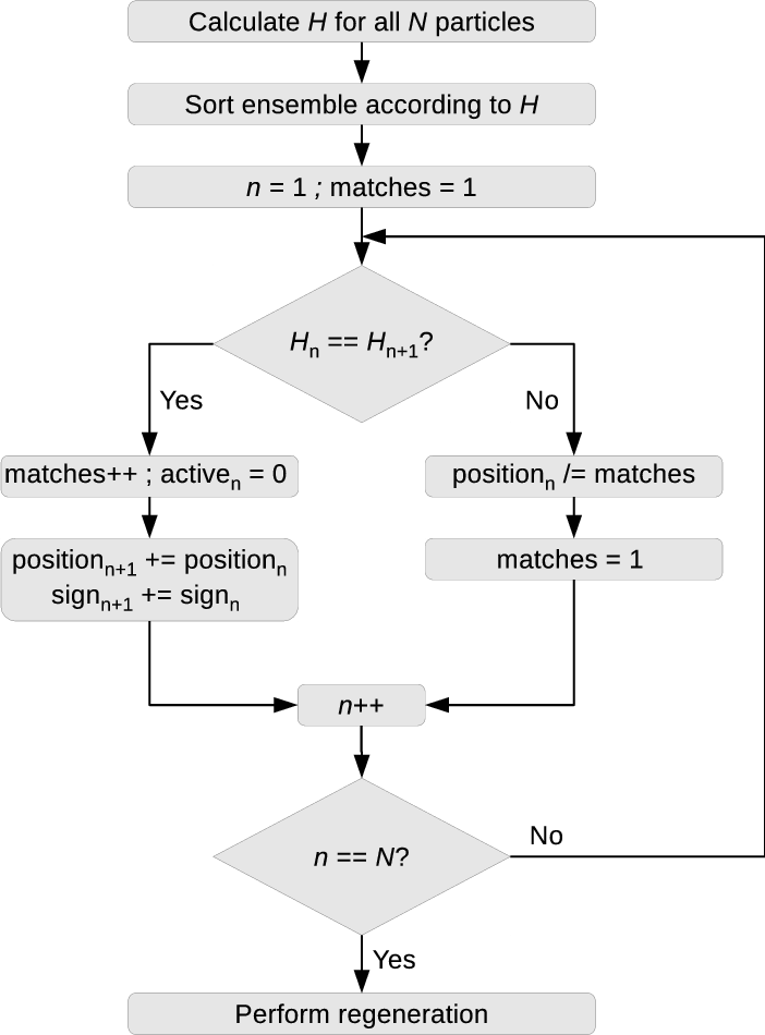
The situation is greatly improved by first sorting the array, representing the particle ensemble, according to the values H. This can be efficiently performed by a
quicksort algorithm which has a  time complexity [141]. In the sorted particle ensemble, all particles in the same cell of the phase space (i.e. the same
value of H) now appear consecutively in the array – this is also beneficial for the memory access speed. The sorted array allows the sum of signs and
mean positions of the particles to be calculated in-place without the need of any additional memory. A flow-chart of the algorithm is shown in
Figure 4.17. The sorted array is iterated, if the value of H for particle n and n + 1 are identical, a ’matches’ counter is incremented, particle n is
deactivated (by a flag) and its sign and position is added to the values of particle n + 1. This process continues until Hn≠Hn+1, then the mean
position of all the particles in the cell corresponding to Hn is calculated by dividing the sum of the positions by the counter which is then reset.
time complexity [141]. In the sorted particle ensemble, all particles in the same cell of the phase space (i.e. the same
value of H) now appear consecutively in the array – this is also beneficial for the memory access speed. The sorted array allows the sum of signs and
mean positions of the particles to be calculated in-place without the need of any additional memory. A flow-chart of the algorithm is shown in
Figure 4.17. The sorted array is iterated, if the value of H for particle n and n + 1 are identical, a ’matches’ counter is incremented, particle n is
deactivated (by a flag) and its sign and position is added to the values of particle n + 1. This process continues until Hn≠Hn+1, then the mean
position of all the particles in the cell corresponding to Hn is calculated by dividing the sum of the positions by the counter which is then reset.
Once the entire ensemble has been covered, the regeneration process commences. The information required for regeneration is stored in the fields for position and sign for particles which are still marked active (activen = 1; cf. Figure 4.17). The new particles are regenerated and stored in the original array, overwriting the particles in the array, which have been deactivated during the annihilation process. This allows the entire annihilation and regeneration process to be completed with an insignificant amount of additional memory.
The trade-off for the small memory footprint of this annihilation algorithm is the additional computation time required to sort the array of the particle ensemble. The calculation of the indices and the regeneration of particles is essentially identical between all the annihilation algorithms presented here. The impact of the sorting on the overall computation time depends on i) the regularity of the annihilation (the generation rate) and ii) the threshold value for the number of particles in the ensemble (N) at which annihilation (sorting) occurs. To characterize the performance impact of the algorithm, the simulation time of two examples are compared with different parameters, as listed in Table 4.3.
The results in Table 4.4 reveal the sorting-based annihilation algorithm increases the computation time between 7% and 19%. In the investigated examples, the peak memory demand of the simulation is not strongly affected by the type of annihilation algorithm, since the chosen resolution of the phase space is coarse and, therefore, the representation of the phase space in memory is small. Indeed, if sufficient memory is available, there are no advantages to using the sort-based algorithm. However, it should be noted that in certain practical cases – as exemplified in Chapter 5 – the memory demands of the conventional annihilation algorithm exceed the capacities of a workstation. Therefore, this algorithm makes two-dimensional Wigner Monte Carlo simulations accessible to users that have limited computational resources. This presents a great step towards a wider adoption of Wigner Monte Carlo simulations.
| A.1 | A.2 | B.1 | B.2 | |
| Max. ensemble size [×106] | 20 | 10 | 5 | 5 |
| Annihilations performed | 23 | 210 | 24 | 33 |
| Simulation time [fs] | 100 | 100 | 100 | 100 |
| Domain [nm] | 100 × 150 | 100 × 150 | 100 | 100 |
Δx [nm] [nm] | 1 | 1 | 1 | 1 |
| Coherence length L [nm] | 30 | 30 | 30 | 60 |
| Reference [s] | Sort-based [s] | Change | |
| A.1 | 2041 | 2425 | +19% |
| A.2 | 1717 | 2028 | +18% |
| B.1 | 427 | 455 | +7% |
| B.2 | 508 | 548 | +8% |
In summary, the annihilation algorithm based on ensemble sorting eradicates the memory demands associated with particle annihilation almost entirely. The trade-off is a slight increase in computation time, which depends on the parameters of the particular simulation problem. The sort-based annihilation algorithm allows two-dimensional Wigner Monte Carlo simulations to be performed on conventional workstations with limited memory resources, also when using high-resolution meshes, which significantly improves the accessibility of multi-dimensional time-dependent quantum transport simulations.
The concept of particle annihilation relies on some approximations and, as has transpired from Section 4.3.1, the process may also introduce undesired numerical side-effects. It is therefore desirable not to perform the annihilation step unless needed (to ensure the total number of particles do not exceed the chosen maximum number).
The conventional approach is to choose (guess) an annihilation frequency (as a multiple of the time step Δt) such that the ensemble maximum is never exceeded. This approach requires some trial-and-error in choosing the most appropriate value, which is very unattractive from a usability point of view. Moreover, a fixed frequency of the annihilation may induce annihilation when it is not needed.
A superior manner to handle the problem is to induce an annihilation only when needed. For this purpose the increase in the number of particles, due to generation (Section 3.7.5), is predicted using the current number of particles and the generation rate (which is known from the WP):

Since the particle generation is a stochastic process (which depends on the generation of random numbers), the exact number of generated particles can only be estimated. The estimate improves as the size of the particle ensemble increases. However, smaller ensemble sizes may occur, e.g. in subdomains of the spatial domain decomposition in parallelized code (discussed in Chapter 5), and then the estimate can deviate considerably from the actual change. Depending on the specific implementation of the algorithm this can be problematic, e.g. when allocating memory in accordance to the growth prediction. It is advisable to overestimate the particle increase. For this reason the reference implementation in ViennaWD uses only the maximum value of γ for all particles, such that