5.4 Algorithm
This section discusses the implementation of the domain decomposition approach, presented in Section 5.3, using MPI. The discussion is made
against the backdrop of the serial algorithm, which has been presented in Chapter 3, and focuses on the additions/changes needed for the
parallelization.
5.4.1 MPI topology
Consider N MPI processes – a master process (process 0) with worker processes (Process 1..(N - 1)) – each assigned to one CPU core. The spatial domain
considered in the simulation, i.e. the dimensions of the structure/device, is divided into N uniformly sized subdomains, one for each process. A
slab-decomposition is used here, as illustrated in Figure 5.1a, but the concepts extend to other space decompositions or higher dimensions.
The subdomains are assigned to processes in a sequential order, thereby inherently allowing each process to ’locate’ the processes treating its
spatially neighbouring subdomains, e.g. Process 2 would be responsible for the subdomain to the left of the subdomain handled by Process 3,
etc.
The MPI communication takes place between each process and its spatially neighbouring subdomains, along with some minimal communication (one character (the
flag) per time step) to the master process for coordination of the annihilation step. Such a decentralized approach avoids a constant querying of the master process,
which – due to increased latency and bandwidth limitations – would impede scaling for increasing numbers of processes. The transfer (communication) of particles
between processes only occurs once at the end of each time-step. This necessitates a small overlap between adjacent subdomains, which serves as buffer to
accommodate particles travelling towards a neighbouring subdomain, until they get transferred to the subdomain at the end of the time step. The exact extent of the
overlap should consider the maximum distance a particle can travel within the chosen time-step as well as its direction of travel. It is desirable to make the overlap
between the subdomains as small as possible to avoid data redundancy which negatively affects the parallel efficiency (in terms of memory
scaling).
5.4.2 Initialization
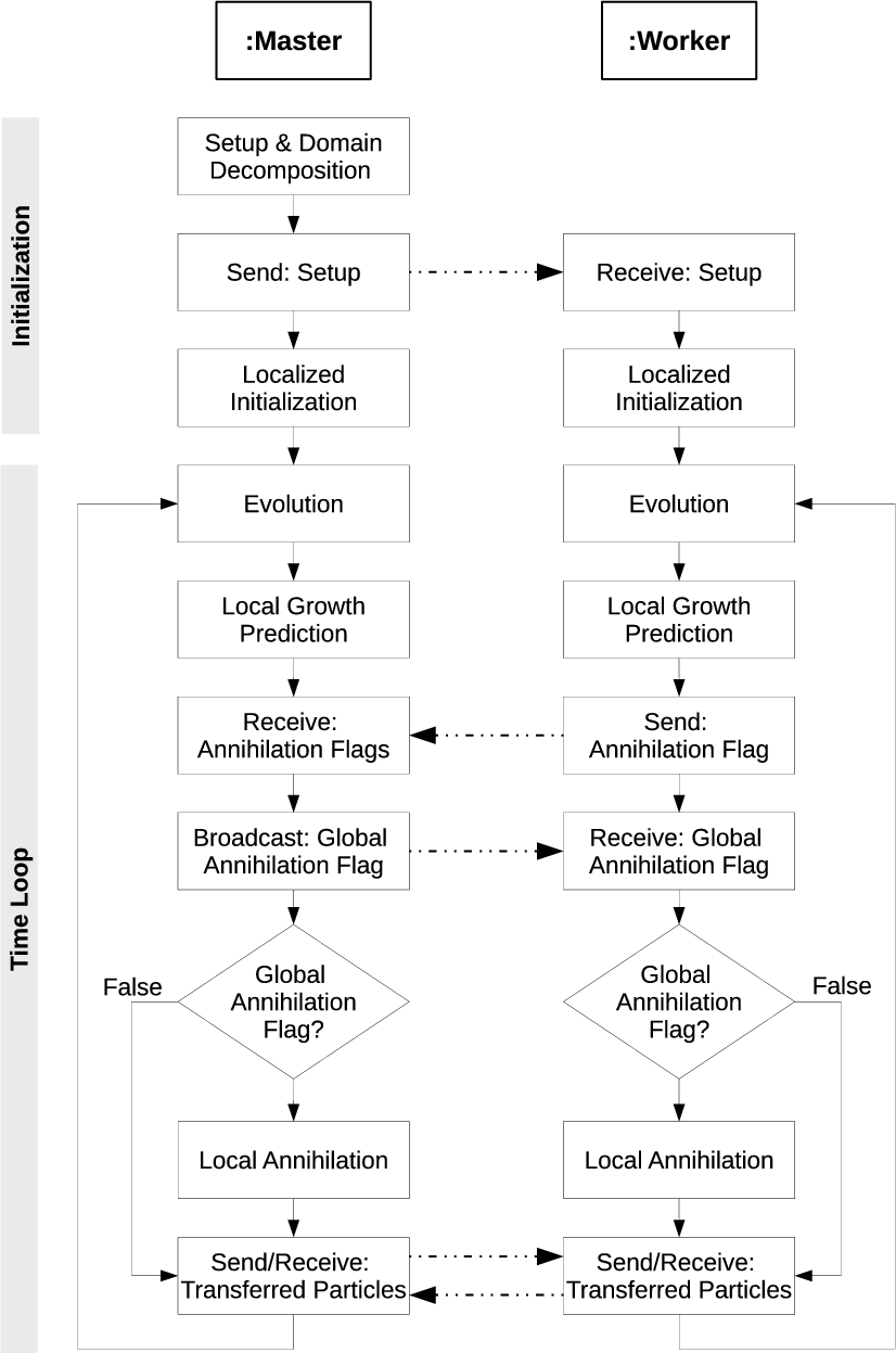
As illustrated in Figure 5.2, the master process performs the initialization of the simulation environment, which entails receiving external input
data (just like in the serial case), performing the discussed domain decomposition and finally communicating this data to the worker processes.
The initial condition for the simulation is given by an (arbitrary) ensemble of particles, which is distributed by the master process amongst the various worker
processes by assigning each particle to an appropriate subdomain based on its position. The particles associated to each subdomain are first collected and then
communicated to the associated worker process by the master process. Furthermore, the master process broadcasts the potential profile and global parameters,
needed for a localized simulation setup, to all worker processes.
After receiving setup parameters and its initial particles ensemble (in case of worker processes), each process initializes localized versions of the required data
structures, specific to its subdomain. Thereby, the memory demands of each process scale down with the number of processes/subdomains. Moreover, the localization
of the WP allows its computation to be distributed amongst the processes, which is beneficial when problems with time-dependent potentials are
considered.
5.4.3 Time loop
After the initialization phase, each process performs the evolution of its ensemble of particles for a single time-step – this is identical to the serial case discussed in
Section 3.7. After the time-step is completed, each process performs a growth prediction for its subensemble of particles, the result of which is
communicated to the master process in the form of an annihilation flag (1-byte character) in order to facilitate a synchronized annihilation
amongst all processes. After the master process has received the flags from all worker processes, it broadcasts a global annihilation flag back
to the worker processes. The global annihilation flag is true, if the annihilation flag of at least one process is true, otherwise it is false. The
annihilation step ensues (or not) locally within each subdomain, depending on the global annihilation flag received. The communication step
associated with the annihilation flag implicitly serves as a synchronization point between the processes, which is required anyway due to the
need to transfer the boundary particles at the end of each time step. Therefore, communicating the annihilation flag does not impede parallel
efficiency.
After the (possible) annihilation step, each process identifies the particles in its subdomain, which qualify for transfer to its adjacent subdomains. These particles are
collected and sent to the appropriate process, which is implicitly known due to the sequential ordering discussed above. Likewise, particles are also received from the
neighbour processes. This communication is non-blocking, however, a synchronization barrier is used to ensure all transfers are complete before the next
time-step commences. Since the processes already will have been synchronized shortly before by the annihilation communication, and the fact
that the execution time of the annihilation procedure does not vary significantly between the processes, this second synchronization is not as
detrimental to the efficiency of the parallelization as it initially appears. The reason for performing the transfer after the annihilation, is that after an
annihilation step the size of the particle ensemble will be significantly smaller, consequently the number of particles to be transferred will have been
reduced.
This sequence of evolution, annihilation and transfer is repeated until the total simulation time has been reached. The simulation results of each process are written
to disks locally by each process, which increases efficiency by avoiding a global reduction step issued by the master process. The simulation results are merged in a
straightforward manner via a separate post-processing step (e.g. on a personal workstation) after the simulation has ended and the reserved computational resources
have been released.