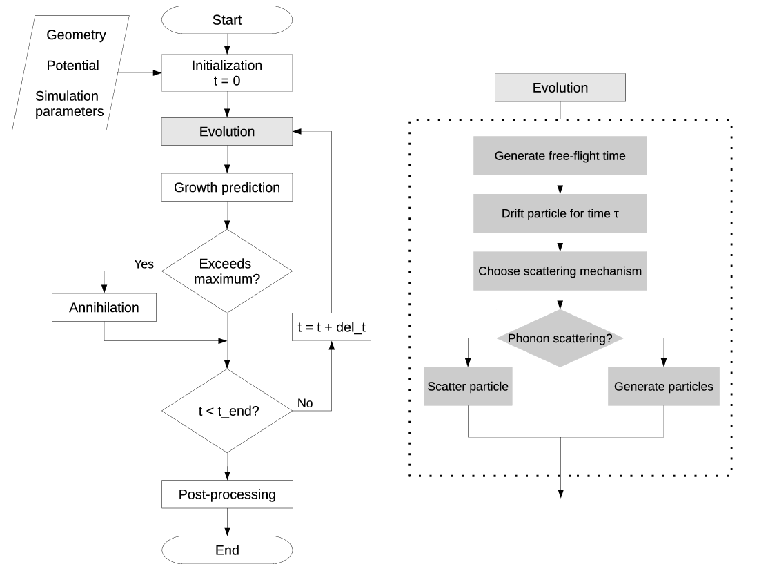
Figure 3.1: Flowchart of a Monte Carlo algorithm to solve the Wigner-Boltzmann equation using the signed-particle method. Particle drift and scattering
and/or generation occur alternately until the end of the simulation is completed.
The preceding sections introduced the Neumann series with which the statistical mean of an arbitrary physical quantity can be represented. The value of the latter can be obtained by stochastic sampling of the Neumann series using numerical particles (each particle represents a sampling). A particle is evolved through free-flight and scattering up to time T, which selects one of the terms in the series. The contribution of the selected term is determined by sampling the integral associated with that term. The mean value of all the sampled values approximates the value of the Neumann series.
An algorithm to perform this task uses the physical interpretation of the various terms to propagate numerical particles along trajectories and scatter them to different wavevectors or spawn additional particles with different wavevectors. This physical interpretation corresponds to the notion of free-flight and scattering used in semi-classical Monte Carlo simulation and allows the adoption of many established algorithms.
The conditions for obtaining a unique solution to (3.25) using this Monte Carlo algorithm and the associated error analysis are formally discussed in [122].
The implementation of this algorithm is discussed in the following subsections, starting with an outline of the basic structure of the algorithm. Thereafter, the basic aspects of the important steps are discussed. A detailed discussion of certain algorithmic aspects is postponed to Chapter 4.
The basic structure of the algorithm to solve the WBE is illustrated in Figure 3.1 and highlights the aspects differentiating the Wigner ensemble Monte Carlo simulation from semi-classical equivalents.
The simulation commences with an initialization step, which receives inputs describing the geometry, potential profile and parameters (e.g. time step, simulation time) used for the simulation and computing the (stationary) Wigner potential. An ensemble of particles representing the initial condition of the evolution problem is initialized. Thereafter, the time loop commences which tracks the trajectories of the particles over time. The position and wavevector of each particle in the ensemble is recorded on a histogram, taking the particle signs into account, at regular time intervals Δt (the observation time), which approximates the distribution function fw(r,k,t).
The time loop consists of the evolution and annihilation modules, which are executed alternately until the total simulation time is reached. The evolution module entails the drift (free-flight) and scattering/generation of particles. Particles are drifted classically according to their momentum value. If a particle experiences a generation event, two new particles are generated and added to the particle ensemble. If a scattering event occurs, the wavevector of the particle is modified according to the selected Boltzmann scattering mechanism. The processes of drift and generation/scattering are repeated in an iterative fashion for all particles in the (growing) ensemble until the end of the time-step is reached.
The annihilation procedure is only performed when needed, i.e. if the size of the particle ensemble will exceed the set maximum in the next time step. This is preferable to performing it at every time step since the annihilation introduces approximations, which can have undesirable effects (discussed in Section 4.3.1). After the annihilation, the remaining particles are regenerated and the time loop continues until the final time is reached.
The integral form for the semi-discrete version of the Wigner equation follows directly from (3.12) by omitting all terms related to phonon scattering and substituting the integral ∫ dk with the summation ∑ q and the wavevector with its discretized form k → qΔk:
Real-valued wavevectors can be retained for the Boltzmann scattering terms, given certain considerations discussed in Appendix B.The calculation of the Wigner potential requires the discretization of the position coordinate, which will be stipulated in Section 4.1.1.
The initial condition from which the evolution starts is represented by an ensemble of N particles. Each particle in the ensemble carries the following attributes:
 (positive real number).
The position and momentum of the particles is initialized according to a chosen distribution or a previously calculated initial condition. The particle signs should only take negative values if the Wigner function, representing the initial condition, is calculated from a physically valid wavefunction.
The Gaussian minimum uncertainty wavepacket is often used as an initial distribution and is defined by
where r0 and k0 represent the mean position and the mean wavevector, respectively; σ is the standard spatial deviation and represents a normalization constant.
Each wavepacket, consisting of many numerical particles, represents a single electron and captures both the particle- and wave-like properties of the electron
[125].
represents a normalization constant.
Each wavepacket, consisting of many numerical particles, represents a single electron and captures both the particle- and wave-like properties of the electron
[125].
Particle drift or free-flight refers to the movement of a carrier, according to Newtonian laws, between scattering events. The electromagnetic forces do not appear explicitly in the Wigner(-Boltzmann) equation, therefore a particle experiences no acceleration due to forces during free-flight and its wavevector remains constant. The position of a particle changes according to


A particle that has completed a scattering event at time t0 will not be scattered again until time τ, i.e. it will undergo free-flight between t0 and τ, with a probability given by

 . Since the particle is not accelerated, the wavevector k is only modified by scattering and
remains constant during the free-flight.
. Since the particle is not accelerated, the wavevector k is only modified by scattering and
remains constant during the free-flight.
Using the concept of self-scattering [126] a value is added to the scattering rate such that it is kept constant  over space and time. Thereby, the need to calculate
the integral in the exponent is avoided and the probability
over space and time. Thereby, the need to calculate
the integral in the exponent is avoided and the probability  is given by

![[0,1]](html_diss_c209x.png) is a uniformly distributed random number. This considerably simplifies the determination of the duration of free-flight:
is a uniformly distributed random number. This considerably simplifies the determination of the duration of free-flight: 
The total scattering rate Γ is calculated once (for a given potential), according to the generation rate (3.4) and the scattering rates given in Appendix A, during the
initialization of the simulator and is retained in a look-up table. The scattering mechanism to be used for a scattering event is randomly selected from the normalized
scattering Table [109] by generating a uniformly distributed random number r ∈![[0,1]](html_diss_c211x.png) . The selected mechanism can either be one of the phonon scattering
mechanisms or a particle generation event.
. The selected mechanism can either be one of the phonon scattering
mechanisms or a particle generation event.
A generation event entails the creation of two additional particles with complementary signs and offsets ℓ1 and ℓ2, with respect to the wavevector k of the generating particle; one particle will have a wavevector k + ℓ1 and the other particle, with the complementary sign (affinity), will have a wavevector k + ℓ2. The Wigner potential (V w; defined in Chapter 2) defines the rate at which particles are generated and the probability distributions used to select momentum offsets.
The two momentum offsets, ℓ1 and ℓ2, are determined by sampling the quantities  and
and  , which represent probabilities, as discussed in Section 3.6.1. Due to the antisymmetry
of the Wigner potential4 :
, which represent probabilities, as discussed in Section 3.6.1. Due to the antisymmetry
of the Wigner potential4 :

![[0,1]](html_diss_c217x.png) is generated to determine the offset ℓ such that
is generated to determine the offset ℓ such that 
The single sampling is attractive from a computational point of view and also a valid approach, if a sufficiently large number of particles is considered in the simulation (law of large numbers). The finite range of the wavevectors considered, however, requires a closer analysis, which is deferred to Section 4.2.
The process of particle generation leads to an exponential increase in the number of particles. The increase in particles within a time step is described by

This numerically debilitating increase in the number of particles is counteracted by the notion of particle annihilation, which keeps the number of particles under control, as discussed in the next section.
The treatment of the conventional phonon scattering mechanisms follows the standard references for Monte Carlo simulation [109, 110]. The equations for the considered scattering mechanisms (specified in Appendix A) theoretically are only valid in bulk semiconductors with a continuous spectrum of energy and wavevectors. The use of the phonon scattering models with a discretized k-grid necessitates some rounding of values, which can introduce an increase in energy. However, experiments have established that the discretization errors accumulate to an insignificant amount over simulation times of interest (several picoseconds). Appendix B can be consulted for details.
The annihilation concept entails dividing the phase space into many cells. Each cell represents a volume  d
d d′ of the phase space, where d (d′) is the
dimension of space (wavevector). Since the wavevector is discretized in the semi-discrete Wigner equation a single value is associated with each
cell.
d′ of the phase space, where d (d′) is the
dimension of space (wavevector). Since the wavevector is discretized in the semi-discrete Wigner equation a single value is associated with each
cell.
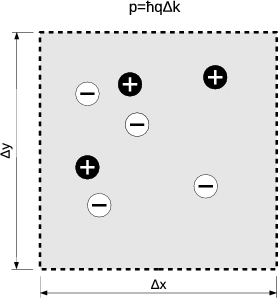
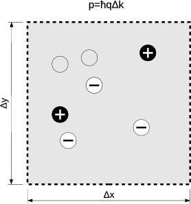
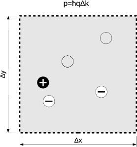
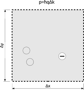
The particles within a given cell are considered to have the same probabilistic future: On average, two particles of opposite sign within a cell will end up in approximately the same place in the phase space and make a contribution to the Wigner function (or any physical quantity), which is equal in magnitude but opposite in sign. Since the particles’ contributions cancel out in the future, they immediately annihilate each other and cease to exist. All the particles within a cell are deemed to be identical and indistinguishable; any positive particle can annihilate any negative particle (and vice-versa). By considering the particles to be identical and indistinguishable avoids the need to keep track of the attributes of each individual particle; instead, the attributes are associated with the cells of the phase space and only the number of particles within the cell is important.
Using the concept of particle annihilation the number of particles and the associated computational burden, is considerably reduced. This is of great importance as it has made the simulations computationally feasible, also in multiple dimensions. The annihilation procedure is illustrated in Figure 3.2 for a two-dimensional cell with a fixed wavevector.
Consider a cell with A particles with a positive sign and B particles with a negative sign, which are summed up to yield a remainder of particles, R = A-B;  particles, each carrying the sign of R, are regenerated within the cell. The
  particles which survive the annihilation procedure should, ideally, recover the
information represented by the
particles which survive the annihilation procedure should, ideally, recover the
information represented by the particles before the annihilation took place. Since the wavevector is quantized and a single value is shared amongst all
particles within a cell, the distribution in the k-space is recovered after annihilation. The positions of the particles, however, are real-valued and
require additional consideration, which will be given in Section 4.3.1. New values for the free-flight time are generated for each particle using the
procedure discussed in Section 3.7.4. Due to the Markovian character of the evolution the values the particles had prior to annihilation need not be
considered.
particles before the annihilation took place. Since the wavevector is quantized and a single value is shared amongst all
particles within a cell, the distribution in the k-space is recovered after annihilation. The positions of the particles, however, are real-valued and
require additional consideration, which will be given in Section 4.3.1. New values for the free-flight time are generated for each particle using the
procedure discussed in Section 3.7.4. Due to the Markovian character of the evolution the values the particles had prior to annihilation need not be
considered.
The models and algorithms presented in the preceding sections (and elsewhere in this work) have been implemented in the WEMC module of the ViennaWD suite of particle-based simulation tools [102]. In addition to the WEMC simulator, ViennaWD includes two additional simulators: i) The Phonon Decoherence (PD) simulator, which uses the single particle Monte Carlo method to simulate the evolution of an entangled quantum state under the influence of phonon scattering in one dimension and ii) the Classical Ensemble Monte Carlo (CEMC) simulator, which allows the self-consistent solution of the BTE for two-dimensional MOSFET structures.
The WEMC simulator is written in C and uses the Message Passing Interface (MPI) for parallel execution in a distributed-memory computing environment (see Chapter 5). ViennaWD is an open source project, publicly available on SourceForge [102], and the development of the WEMC simulator presents a major contribution to enabling other researchers to use and investigate Wigner-based simulation for time-resolved quantum transport.
User interaction with the WEMC simulator is facilitated through input files, which are specified as command line arguments at execution. The simulation parameters, like time step and simulation domain, are specified using a text-based input file, implemented using scripts written in Lua [127]. The potential profile and/or initial condition can also be specified with text files, using a simple text format. Alternatively, the potential profile and the initial conditions can be generated directly in the simulator with analytical functions and distributions.
Post-processing of the output data is handled by Python scripts, which merge data files (if needed) and execute further scripts, which generate the requested graphical output. Plots of output data, e.g. density or k-distribution, are automatically generated (if selected) using gnuplot scripts.
The complete documentation on the use of the simulator has been made available through the ViennaWD user manual [102].