2.2.2 Feature-Scale Transport

Plane ${\mathcal {P}}$ together with surface ${\mathcal {S}}$ represent the boundary of the feature-scale region (see Figure 2.1). If the arriving flux distribution ${\Gamma}_{\text{src}}$ is known at ${\mathcal {P}}$ , and for all surface points ${\vec{x}}\in{\mathcal{S}}$ the reemitted flux distribution ${\Gamma}_{\text{re}}={\Gamma}_{\text{re}}({\vec{x}};{q}, {\vec{\omega}}, {E})$ is given, the particle transport through the feature-scale region is well-defined. This allows the determination of the arriving angular energy particle flux distribution ${\Gamma}={\Gamma}({\vec{x}};{q}, {\vec{\omega}}, {E})$ on the surface ${\mathcal {S}}$ , which principally defines the surface rates. The dependence of the reemitted flux distribution ${\Gamma}_{\text{re}}$ on the local arrival flux distribution ${\Gamma}$ will be discussed later.

For most processes the frequency of particle-particle collisions at feature-scale is negligible relative to particle-surface collisions [21]. For comparison, according to (2.4) the mean free path for an ideal gas at room temperature ( ${T}\approx\SI{300}{\kelvin}$ ) and atmospheric pressure ( ${P}\approx\SI{100}{\kilo\pascal}$ ) is approximately $\SI{60}{\nm}$ , which is of the same magnitude as typical sizes of modern structures. However, most dry processes operate at much lower pressures, where the mean free path is much larger than typical feature sizes. This validates the assumption of ballistic transport within the feature-scale region.

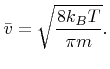
The average particle velocities are usually much larger than the surface rates. Kinetic theory gives the mean particle velocity ${\bar{{v}}}$ of an ideal gas as [22]

$${\bar{{v}}}=\sqrt{\frac{8{k_B}{T}}{\pi{m}}}.$$ (2.13)

For typical temperatures ${T}$ and molecular weights ${m}$ the average velocity is larger than $\SI{100}{\metre\per\second}$ . In comparison, the surface rates in most processes are well below $\SI{1}{\micro\metre\per\second}$ . As a consequence, the surface can be regarded to be constant and the travel time of particles can be neglected for calculating the arrival flux distribution at a certain time.

In the ballistic transport regime the particle trajectories of neutral particles are straight lines. For charged particles, such as ions, electromagnetic forces must be incorporated. Incident ions charge insulating layers, such as SiO$_2$ . This leads to a static electric field influencing the ion trajectories [30,48]. If the electric field becomes strong enough, the trajectories can be disturbed significantly, which affects the final profile. For example, charging is an essential mechanism for the notching effect which can be observed, if polysilicon-on-insulator structures are overetched [48]. Despite the importance of charging for the description of some effects, this work does not incorporate electromagnetic forces for the intra-feature particle transport. However, as will be outlined in Chapter 7 the main ideas of this work can be extended to incorporate electrostatic fields.

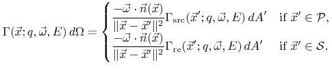
In the absence of electromagnetic forces the trajectories of all particles are straight lines. The particles which arrive at a surface point ${\vec{x}}\in{\mathcal{S}}$ with incident direction ${\vec{\omega}}$ can either originate from ${\mathcal {P}}$ or from the surface itself due to reemission, as shown in Figure 2.1. Thus, the particle transport at feature-scale can be described by

$${\Gamma}({\vec{x}};{q},{\vec{\omega}}, {E})\,{d}{\Omega}= \begin{... ...omega}},{E})\,{d}{A}'} & \text{if} \ {\vec{x}}'\in{\mathcal{S}}. \\ \end{cases}$$ (2.14)

Here ${\vec{x}}'\in{\mathcal{P}}\cup{\mathcal{S}}$ is the point seen from point ${\vec{x}}$ in direction $-{\vec{\omega}}$ , thus ${\vec{\omega}}=\frac{{\vec{x}}-{\vec{x}}'}{\lVert{\vec{x}}-{\vec{x}}'\rVert}$ . ${d}{A}'$ is an infinitesimal surface element of ${\mathcal {S}}$ or ${\mathcal {P}}$ around ${\vec{x}}'$ . ${\vec{n}}({\vec{x}})$ is the surface normal at point ${\vec{x}}$ .