4.8.2 Graph Setup Algorithm

If the H-RLE data structure is used, the utilization of the following properties allows the setup of a reduced graph which already combines several grid points within a vertex, and consequently, for which it is much easier to determine its connected components:

• As already mentioned in Section 3.5.4 the H-RLE data structure leads to a segmentation of the grid. Such a segment is either a defined grid point or an undefined run which combines one or more undefined grid points with the same LS sign (compare Figure 3.7).

• All grid points within a segment are connected. The connectivity follows for undefined runs from the fact that all contained grid points are neighbored and have the same sign. Hence, if any points of two different neighboring segments are connected, all of their points are also connected to each other.

• Two segments are neighbored, if and only if at least one of their corresponding first points is a neighbor to the other segment. The first point of a segment means the first point according to the lexicographical order given by the HRLE data structure. Its index vector is equal to the start index vector of a basic iterator positioned at the corresponding segment. As a consequence, it is sufficient to obtain all required connectivity relations between segments, by testing the neighboring points of all first points for connectivity.

To set up the reduced graph an array is needed to store a reference to the corresponding vertex for each segment in the H-RLE data structure. Using a basic iterator the H-RLE data structure is sequentially traversed and for each segment the following two tasks are performed:

1. The neighboring points of the first grid point in the current segment are tested for connectivity. If none of the corresponding connected neighbor segments is assigned to a vertex, a new vertex is inserted into the graph to which the current segment is assigned. Otherwise, the current segment is assigned to an arbitrary vertex to which a connected neighbor belongs.

2. All connected neighbor segments which do not belong to any vertex are assigned to the same vertex as the current segment. If there is a connected neighbor belonging to a different vertex, a new edge between the corresponding vertices is inserted in the graph.

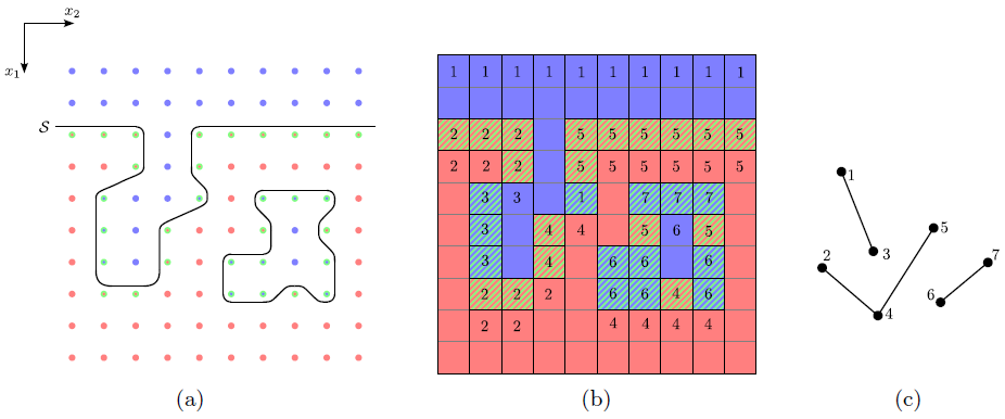
Figure 4.17 shows an example with a LS representing a geometry with a void. After the procedure each segment is assigned to a vertex of the reduced graph. Due to the incorporation of connectivity relations during the setup, the number of vertices of the reduced graph is usually only a fraction of the number of defined grid points.

Figure 4.17: (a) The surface ${\mathcal {S}}$ of a geometry with a void. Blue and red points have positive and negative LS values, respectively. Defined grid points are also colored green. (b) The corresponding segments of the H-RLE data structure. Their numbers give the vertex of the reduced graph they are assigned to. (c) The reduced graph which is set up to find the connected components.