5.3.1 Power Cosine Distribution

First the power cosine distribution as introduced in (2.6) is considered, where 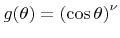${g}({\theta})=\left(\cos{\theta}\right)^{\nu}$ with ${\nu}>0$ . Thus the probability density function for the polar angle is given as

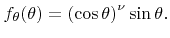$${f}_{\theta}({\theta})=\left(\cos{\theta}\right)^{\nu}\sin{\theta}.$$ (5.36)

Calculating the cumulative distribution function results in

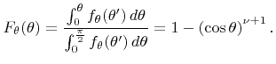$${F}_{\theta}({\theta}) = \frac{\int_{0}^{{\theta}}{f}_{\theta}({\... ...{f}_{\theta}({\theta}') \,{d}{\theta}} = 1-\left(\cos{\theta}\right)^{{\nu}+1}.$$ (5.37)

A variate obeying an arbitrary distribution can be obtained using the inversion method [25]. A uniformly distributed variate ${u}$ on $\left[0,1\right]$ mapped by the inverse cumulative distribution function leads to the desired distribution [115]

$${\theta}={F}_{\theta}^{-1}({u})=\arccos\left(\sqrt[{\nu}+1]{1-{u}}\right).$$ (5.38)

Since $1-{u}$ is uniformly distributed on $\left[0,1\right]$ as well, the random polar angle can also be generated by [66]

$${\theta}=\arccos\left(\sqrt[{\nu}+1]{{u}}\right).$$ (5.39)

Algorithm 5.2 summarizes the generation of a random polar angle following the probability density function (5.36).