3.3.1 NAOS Modeling

In order to model NAOS, experimental results from several publications from the group of Asuha et al. at the Institute of Scientific and Industrial Research at Osaka University and from Imai at al. at the Display Technology Development Group at Sharp Corporation are analyzed [88], [89], [103].

Figure 3.7: Phase diagram of the Nitric acid (HNO$_3$/H$_2$O) system.

The phase diagram of the HNO$_3$/H$_2$O system is shown in Figure 3.7.

3.3.1.1 Azeotropic NAOS Method

For the azeotropic NAOS method the silicon substrate is submerged in a nitric acid (HNO$_3$) liquid at its boiling temperature. The method is usually performed with a 61wt% concentration of HNO$_3$ at the boiling temperature of 112 $^\textrm {o}$C. An alternative is a 68wt% concentration (location C in Figure Figure 3.7), at the boiling temperature of 120.7 $^\textrm {o}$C. The chemical reaction which takes place in order to generate the oxygen required for the oxidation process is

$$2HNO_3 \rightarrow 2NO + H_2O + 3O$$ (94)

The maximum thicknesses of SiO$_2$ reached are 1.2nm and 1.4nm by oxidation with 61wt% and 68wt% HNO$_3$, respectively within 10 minutes, while prolonged oxidation does not increase the SiO$_2$ thickness. However, until the final thickness is reached, there is still a time dependence on the immersed oxide thickness. This is shown in Figure 3.8a where the thickness of the NAOS oxide is plotted with respect to the immersion time at an ambient temperature of 25 $^\textrm {o}$C immersed in a 61wt% HNO$_3$ solution. Similarly, the temperature dependence on oxide thickness is shown in Figure 3.8b. The thicknesses obtained are after immersion for 10 minutes in a 61wt% HNO$_3$ solution. At the final experimental dot, at a temperature of 112 $^\textrm {o}$C, the oxide reaches its maximum thickness of 1.3nm within the 10 minutes provided.

Figure 3.8: The dependence of immersion time and temperature on the growth of NAOS oxide submersed in a 61wt% HNO$_3$ solution.

(a) Time dependence (T=25$^o$C).	(b) Temperature dependence (t=10 min).

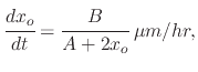
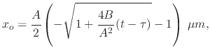
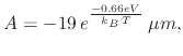
The model must take into account both the influence of immersion time and temperature. From observing Figure 3.8, a linear-parabolic type of relationship seems to dominate the NAOS type of oxidation. The presented model proceeds to fit the experimental data into the linear-parabolic model for the oxide rate

$$\cfrac{dx_{o}}{dt}=\cfrac{B}{A+2x_{o}}\:\mu m\slash hr,$$ (95)

where $x_o$ is the oxide thickness in m, $B$ and $A$ are rate constants analogous to those suggested for the Deal-Grove model with different values. As with the Deal-Grove model, the rate constants have an Arrhenius-type relationship with regard to temperature

$$A=-19\,e^{\frac{-0.66eV}{k_{B}\,T}}\:\mu m,$$ (96)

$$B=1.32\,e^{\frac{-0.132eV}{k_{B}\,T}}\:\mu m^2\slash hr,$$ (97)

where $k_B$ is the Boltzmann constant in eV/K and $T$ is the temperature in Kelvin. Integrating (3.24), an explicit expression for the oxide thickness $x_o$ can be found

$$x_{o}=\cfrac{A}{2}\left(-\sqrt{1+\cfrac{4B}{A^{2}}\left(t-\tau\right)}-1\right)\:\mu m,$$ (98)

where $\tau$ is an adjustment coefficient which accounts for the initial oxide observed in Figure 3.8a. In Figure 3.8, the model is shown to have a good fit to the measured results from [103].

3.3.1.2 Vapor NAOS Method

The vapor NAOS oxidation method should be performed at temperatures above 200$^o$C when the Nitric acid HNO$_3$ is in a vapor phase. The chemical reaction which takes place in order to generate the oxygen required for the oxidation reaction is

$$2HNO_3 \rightarrow NO_2 + NO + H_2O + 2O.$$ (99)

In Figure 3.9 the thickness of the SiO$_2$ layer is plotted as a function of oxidation time for various temperatures (300 $^\textrm {o}$C, 400 $^\textrm {o}$C, 450 $^\textrm {o}$C, and 500 $^\textrm {o}$C). At these temperatures, thermal oxidation would not be able to grow layers larger than the native oxide due to the oxidants not having enough energy to diffuse through the oxide network. The oxide thickness appears to increase with increased time; however the oxidation rate tends to decrease. This parabolic relationship suggests that the diffusion of oxygen atoms through the growing oxide is the rate-determining step.

Figure 3.9: Plots of the SiO$_2$ thickness with respect to the oxidation time at different temperatures when the vapor NAOS method is used. Dots are experimental results from [103] and lines are the results of the presented empirical model.

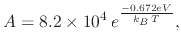
An empirical model which is to follow the oxide growth due to vapor NAOS oxidation must take into account the temperature and time dependence on the oxide thickness. At first the relationship between the oxide thickness and oxidation time is shown to be logarithmic

$$x_{o}=A\,\ln(t)+B\:nm,$$ (100)

where $t$ is the oxidation time and $A$ and $B$ are temperature dependent parameters

$$A=8.2\times10^{4}\,e^{\frac{-0.672eV}{k_B\,T}},$$ (101)

$$B=\cfrac{1060\,\nm\,K}{T}-2.95\times10^{5}\,e^{\frac{-0.673eV}{k_{B}\,T}}\:nm,$$ (102)

where $k_B$ is the Boltzmann constant in eV/K and $T$ is the temperature in Kelvin. The fit of the empirical model to the measured data from [103] is shown in Figure 3.9.