The pure diffusion equation is solved with the finite element and the finite volume method using AMIGOS [128]. This allows the comparison of the solutions on identical meshes with the same linear solver. A Gaussian profile is used as the initial distribution. In two dimensions correct and identical results are obtained with both methods on Delaunay meshes. In three dimensions the finite volume method still achieves correct results on a Delaunay mesh as expected. However, the finite element method fails on the same three-dimensional Delaunay mesh. Even for such a simple test problem the finite element solution strongly violates the maximum principle. The resulting concentration reaches negative values in some areas. These areas spread out in time and the absolute value of the emerging negative concentrations is much larger than the minimal initial concentration. The relative error between the solutions of the two methods oscillates strongly and is large in regions where the concentration is negative. These negative concentrations are particularly annoying for diffusion applications in semiconductor process simulation where the concentration varies many orders of magnitude within a small area.
In the following the observed effects are investigated in terms of mesh requirements and simple mesh examples are constructed where the finite element method can be applied successfully to the diffusion problem.
The examples were constructed by exploiting an ortho-product point distribution. A cube defined by eight points can be tetrahedralized in two qualitatively different ways.
![\includegraphics [width=4cm]{ppl/matrixt6.ps}](img124.gif)
|
Suitable meshes for simulation are then built by stacking a large number of
such tessellated cubes. The typical characteristics of each tessellation
type are thereby conserved.
Hence, both meshes are global Delaunay meshes and yet only one satisfies
Crit. 3.3.
The two fundamentally different meshes based on an identical
ortho-product point cloud are depicted in Fig. 3.11 and Fig. 3.12.
The finite element simulation on the ![]() type Delaunay mesh results in
negative concentrations as was previously pointed out.
The
type Delaunay mesh results in
negative concentrations as was previously pointed out.
The ![]() type Delaunay mesh which fulfills Crit. 3.3
indeed succeeds to yield the required entries in the stiffness matrix and
the concentrations remain positive at any time during the transient
simulation.
type Delaunay mesh which fulfills Crit. 3.3
indeed succeeds to yield the required entries in the stiffness matrix and
the concentrations remain positive at any time during the transient
simulation.
The most important fact however is shown by the third example.
Further exploiting the ortho-product point set and its ![]() type
tessellation with slightly shifted points in certain locations results
in a non-Delaunay mesh which still satisfies
Crit. 3.3.
Figure 3.9 shows an instance of the mesh consisting of eight
cubes. The point in the middle has been shifted.
The Delaunay criterion is violated, because the circumspheres of
several unmodified tetrahedra contain the shifted point in its interior.
The dashed line in the figure marks two of the non-Delaunay triangles.
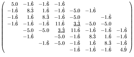
The simulation using AMIGOS for the entire mesh
(Fig. 3.13) shows, that the requirements for the stiffness matrix
are fulfilled. For example one can consider the edge
type
tessellation with slightly shifted points in certain locations results
in a non-Delaunay mesh which still satisfies
Crit. 3.3.
Figure 3.9 shows an instance of the mesh consisting of eight
cubes. The point in the middle has been shifted.
The Delaunay criterion is violated, because the circumspheres of
several unmodified tetrahedra contain the shifted point in its interior.
The dashed line in the figure marks two of the non-Delaunay triangles.
The simulation using AMIGOS for the entire mesh
(Fig. 3.13) shows, that the requirements for the stiffness matrix
are fulfilled. For example one can consider the edge ![]() in
Fig. 3.9.
This edge is shared by elements which contain the shifted point and
which are non-Delaunay.
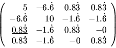
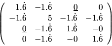
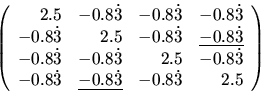
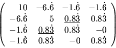
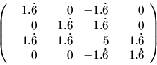
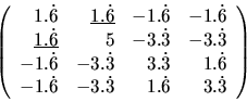
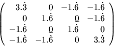
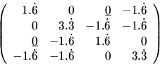
The matrix contributions of the six elements which are
adjacent to this edge are given in Fig. 3.10.
The first two matrices belong to the elements with the shifted point,
and indeed possess undesirable positive off-diagonal entries.
The last two matrices however belong to very well shaped elements
which are able to compensate the overall sum.
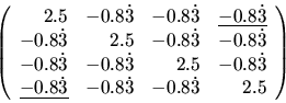
The resulting entry in the global stiffness matrix for the edge
in
Fig. 3.9.
This edge is shared by elements which contain the shifted point and
which are non-Delaunay.
The matrix contributions of the six elements which are
adjacent to this edge are given in Fig. 3.10.
The first two matrices belong to the elements with the shifted point,
and indeed possess undesirable positive off-diagonal entries.
The last two matrices however belong to very well shaped elements
which are able to compensate the overall sum.
The resulting entry in the global stiffness matrix for the edge
![]() equals
equals
![]() .
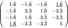
Again, the concentrations do not reach negative values at all times.
The shifting of a point introduces obtuse dihedral angles and positive
contributions to off-diagonal elements of the stiffness matrix.
However, Crit. 3.3 is satisfied and the stiffness
matrix remains an M-matrix.
.
Again, the concentrations do not reach negative values at all times.
The shifting of a point introduces obtuse dihedral angles and positive
contributions to off-diagonal elements of the stiffness matrix.
However, Crit. 3.3 is satisfied and the stiffness
matrix remains an M-matrix.
|
![\includegraphics [height=6cm]{ppl/myMAT1.ps}](img137.gif)
![\includegraphics [height=6cm]{ppl/my.ps}](img138.gif)
![\includegraphics [height=6cm]{ppl/myorg.ps}](img139.gif)
|
![\includegraphics [width=0.77\textwidth]{ppl/eureka3.eps}](img130.gif)