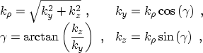
The processes ECB and HVB shown in Fig. 3.1 can be investigated
considering an energy barrier as shown in Fig. 3.2. Two
semiconductor or metal regions are separated by an energy barrier with barrier
height
 , measured from the FERMI energy to the conduction band
edge of the insulating layer. Electrons tunnel from Electrode 1 to Electrode
2. The distribution functions at both sides of the barrier are indicated in
the figure.
, measured from the FERMI energy to the conduction band
edge of the insulating layer. Electrons tunnel from Electrode 1 to Electrode
2. The distribution functions at both sides of the barrier are indicated in
the figure.
Figure 3.2:
Energy barrier with two electrodes which can
be used to describe the ECB or HVB processes.
|
|
In the following derivation some assumptions will be made which are necessary
to allow an easy incorporation of the model in a device simulator. These are:
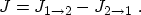
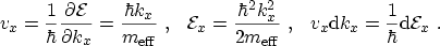
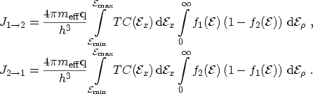
The net tunneling current density from Electrode 1 to Electrode 2 can be
written as the net difference between current flowing from Side 1 to Side 2 and
vice versa [96,97]
 |
(3.2) |
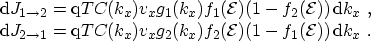
The current density through the two interfaces depends on the perpendicular
component of the wave vector  , the transmission coefficient
  , the
perpendicular velocity
, the
perpendicular velocity  , the density of states
  , and the distribution
function at both sides of the barrier:
, and the distribution
function at both sides of the barrier:
 |
(3.3) |
In this expression it is assumed that the transmission coefficient only
depends on the momentum perpendicular to the interface. The density of
states  is
is
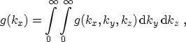 |
(3.4) |
where
 denotes the three-dimensional density of states in the
momentum space. Considering the quantized wave vector components within a cube of
side length
denotes the three-dimensional density of states in the
momentum space. Considering the quantized wave vector components within a cube of
side length 
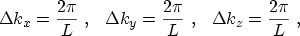 |
(3.5) |
yields for the density of states within the cube
 |
(3.6) |
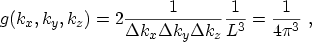
where the factor 2 stems from spin degeneracy. For the parabolic dispersion
relation (3.1) the velocity and energy components in tunneling
direction obey
 |
(3.7) |
Hence, expressions (3.3) become
 |
(3.8) |
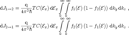
Using polar coordinates for the parallel wave vector components
 |
(3.9) |
the current density evaluates to
 |
(3.10) |
In these expressions the total energy
 has been split into a longitudinal
part
has been split into a longitudinal
part
 and a transversal part

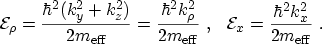 |
(3.11) |
Evaluating the difference
 , the net current
through the interface equals
, the net current
through the interface equals
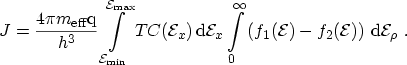 |
(3.12) |
This expression is usually written as an integral over the product of two
independent parts which only depend on the energy perpendicular to the
interface: the transmission coefficient
 and the supply function
 :
:
 |
(3.13) |
which is the expression known as TSU-ESAKI formula. This model has been
proposed by DUKE [98] and was used by TSU and ESAKI
for the modeling of tunneling current in resonant tunneling
devices [99]. The values of
 and
and
 depend on the
considered tunneling process:
depend on the
considered tunneling process:
- Electrons tunneling from the conduction band (ECB):
is the highest conduction band edge of the two electrodes,
is the highest conduction band edge of the dielectric.
- Holes tunneling from the valence band (HVB):
is the absolute
value of the lowest valence band edge of the electrodes,
is the
absolute value of the lowest valence band edge of the dielectric. The sign of
the integration must be changed.
- Electrons tunneling from the valence band (EVB):
is the lowest
conduction band edge of the two electrodes,
the highest valence band
edge of the two electrodes. It must be checked if
 .
.
The next sections concentrate on the calculation of the supply function and the
transmission coefficient.
A. Gehring: Simulation of Tunneling in Semiconductor Devices
![\includegraphics[width=.5\linewidth]{figures/barrierElectrons}](img272.png)