3.5 Transmission Coefficient Modeling

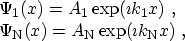
Now that the shape of the energy barrier has been treated, the calculation of the quantum-mechanical transmission coefficient of such a barrier can be investigated. The transmission coefficient $TC$ is defined as the ratio of the quantum-mechanical current density (2.16) due to an incident wave in Region 1 and a transmitted wave in Region N, see Fig. 3.9. The assumption of plane waves in both regions^3.5

$$\begin{array}{l} \Psi_{1}(x) = A_{1} \exp(\imath k_1 x) \ , \... ...thrm{N}}\exp(\imath \ensuremath{k_\mathrm{N}}x) \ , \end{array}$$ (3.53)

leads to the transmission coefficient

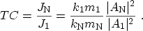$$TC = \frac{ \ensuremath{J_\mathrm{N}}}{J_1} = \frac{k_1 m_1}{\ens... ...\mathrm{N}}} \frac{\vert\ensuremath{A_\mathrm{N}}\vert^2}{\vert A_1\vert^2} \ .$$ (3.54)

The wave function amplitudes $A_1$ and $\ensuremath{A_\mathrm{N}}$ can be found by solving the stationary SCHRÖDINGER equation (2.13) in the barrier region. This can be achieved by various methods. The WENTZEL-KRAMERS-BRILLOUIN approximation can be applied either analytically for a linear barrier, or numerically for arbitrary barriers. GUNDLACH's method can be used for a single linear energy barrier, while the transfer-matrix and quantum transmitting boundary methods are applicable for arbitrary-shaped barriers. The transfer-matrix method can be applied using either constant or linear potential segments as shown in Fig. 3.9. The different methods will be described in this section and a brief comparison at the end summarizes their advantages and shortcomings.

Figure 3.9: The energy barrier of a single-layer dielectric. The potential energy $W(x)$ may either be the conduction band or the valence band energy, depending on the tunneling process. The linear and constant potential approximations refer to the transfer-matrix method described in Section 3.5.3.

Subsections

• 3.5.1 The WENTZEL-KRAMERS-BRILLOUIN Approximation
• 3.5.2 The GUNDLACH Method
• 3.5.3 Transfer-Matrix Method
  • 3.5.3.1 Piecewise-Constant Potential
  • 3.5.3.2 Piecewise-Linear Potential
  
  
• 3.5.4 Quantum Transmitting Boundary Method
• 3.5.5 Comparison

A. Gehring: Simulation of Tunneling in Semiconductor Devices