Since the spin injection efficiency’s upper limit is the polarization in the ferromagnetic semiconductor, one needs to further investigate the peculiarities of the spin signal in silicon if the spin is injected through only a charge neutral or space-charge layer. One can solve the same set of spin transport equations either by adjusting the up- and down-spin concentrations or up- and down-spin current densities at one of the boundaries (i.e. left boundary), to impose a charge-neutral; a charge-accumulated; and a charge depleted source. The schematic is shown in Figure 5.12.
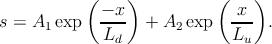
The general solution for the spin density in the bar (c.f. Figure 5.12) can be considered to be in the form [173]
|
| (5.44) |
Here, the constants
The polarizations for the spin current density and the spin density at the
injection boundary are  and
and  respectively. The channel length
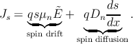
The expression for the spin current density can be obtained from Equation 5.22a and Equation 5.22b
 | (5.46) |
Thus, by using Equation 5.44 one can write
![[( ) ( ) ( ) ( ) ]
Js = q μnE˜ 1 + -VT-- A2 exp x-- + 1 - -VT-- A1 exp - x- .
˜ELu Lu ˜ELd Ld](diss_htm387x.png) | (5.47) |
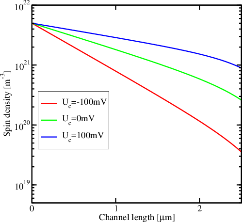
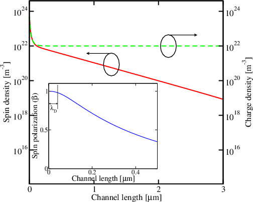
The spin density distribution
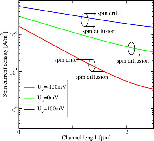
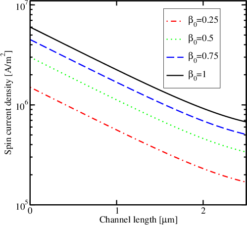
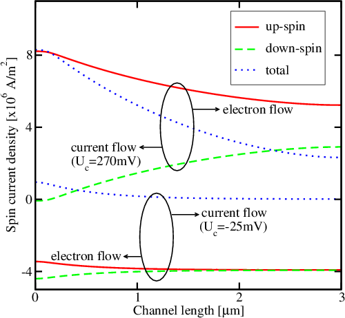
Figure 5.15 examines the variation of the spin current density
A functional spintronic device also involves the reverse process of spin injection, i.e. the extraction of spin-polarized electrons from the semiconductor to a ferromagnetic structure. One can investigate spin extraction from a non-magnetic semiconductor like silicon into the ferromagnet in the regime where the degree of spin polarization is very high. For the analysis of the spin extraction phenomenon, the detailed structure of the interface is not very important, and one can solve the spin transport equations for the semiconductor region instead [191]. The electrons, flowing from the silicon side and entering in the magnet, are supposed to be unpolarized. Now, if the structure is a ferromagnetic half-metal [103], then it accepts only one spin orientation (e.g. up-spin electrons). In such a case, a cloud of down-spin electrons is formed in silicon near the relevant boundary, as those can not enter in the ferromagnet unless undergoing a spin flip. The current in the bar increases the cloud, and eventually reaches its maximum, when the silicon region near the junction becomes completely depleted of the electrons with the same direction of spins (i.e. up-spins) as in the ferromagnet. This phenomenon is known as spin-blockade [191]. This signifies that a further increase of the steady-state current through the junction will not be possible.
In order to estimate this critical current density represented as  solely determines the
transport [191]. Then, one can assume the spin density for the spin extraction
model in the form of [191]
solely determines the
transport [191]. Then, one can assume the spin density for the spin extraction
model in the form of [191] 

 , where
![[( ) ( ) ]
˜ VT-- --x-
Js = qμnE 1 - ˜EL ′ (- A1) exp L ′ .](diss_htm395x.png) | (5.48) |
Henceforth at the spin extraction boundary,
![[( ) ]
J = - qμ ˜E 1 - -VT- A .
s0 n ˜EL ′ 1](diss_htm396x.png) | (5.49) |
The spin current density and the charge current density are related by
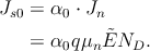 | (5.50) |
Because the electric field
![[ ( VT ) ]
- qμn ˜E 1 - ---- A1 = α0q μn ˜END,
E˜L ′](diss_htm398x.png) | (5.51) |
which eventually yields to
![[( V ) ]
--T- - 1 A1 = α0ND,
E˜L ′](diss_htm399x.png) | (5.52) |
and therefore,
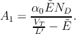 | (5.53) |
If the expression for the up-stream diffusion length is put in Equation 5.53,  . Since the maximum possible spin polarization
can only be 100%, the maximum possible value for
. Since the maximum possible spin polarization
can only be 100%, the maximum possible value for
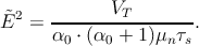 | (5.54) |
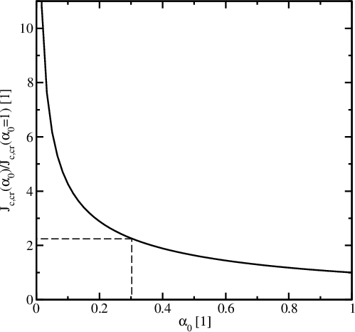
Finally, one can write the expression for the critical current density
 | (5.55) |
A fully polarized (unpolarized) spin current pertains to
Figure 5.17 depicts the critical current density at the spin-blockade.
In order to lift the charge neutrality constraint, one can adjust the up(down)-spin
concentrations
 | (5.56) |
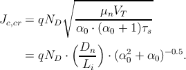
Now, if the maximum value for the spin density polarization
![[ n ] [ exp(MCh-) ]
↑0 = ND VT ,
n↓0 0](diss_htm406x.png) | (5.57) |
and thus making
 | (5.58) |
Therefore, one can inject (release) up-spin and hence charge at the same time. This way it is possible to describe
Via Equation 5.57 a considerable spin and charge accumulation (depletion) at
the interface can be introduced and spin will diffuse out of this region. Non-zero
values of
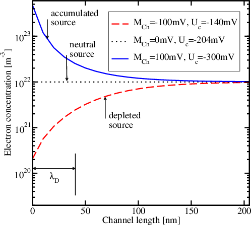
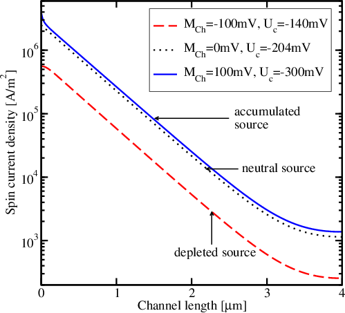
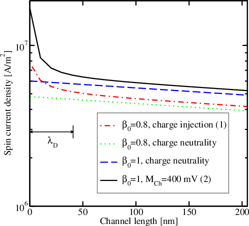
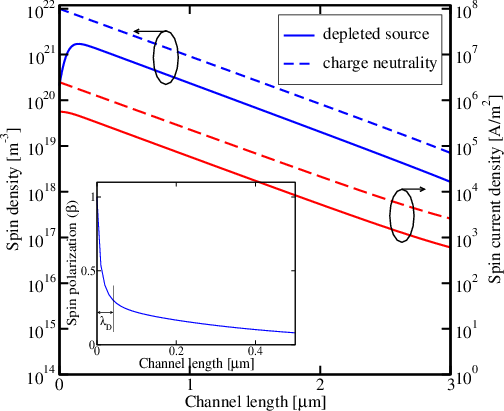
Figure 5.19 depicts how the charge accumulation (depletion) causes the pile
up (reduction) of the carriers near the left boundary and through the
channel. As found previosuly, this pile up persists only up to the screening
region characterized by the Debye length
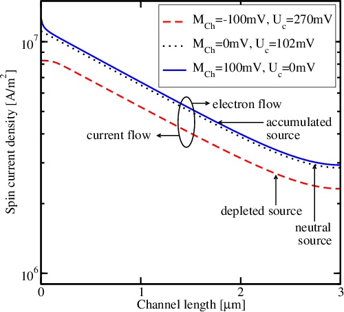
To scrutinize any further enhancement in the spin current density
Up to now it has been predicted that at a fixed boundary spin density
polarization


