 :
: The last section has been devoted to the possible physical explanations for the charge trapping process in NBTI. The involved mechanisms, such as quantum mechanical tunneling for instance, are characterized by their stochastic nature. This means that one must deal with probabilities instead of pre-determined transition times for the trapping events. Such problems can be best handled within the framework of homogeneous continuous-time Markov chain theory [131], which rests on the assumption that the transition rates do not depend on the past of the investigated system.
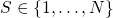
The continuous time Markov chain theory presumes a set of discrete states
:

 are the time-dependent occupation probabilities, which fulfill the
normalization condition
are the time-dependent occupation probabilities, which fulfill the
normalization condition 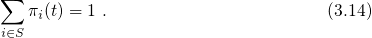
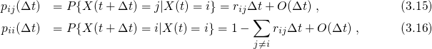
 equals unity. The time-dependent probability
  for a transition from state
 to state
  can be formulated as where
  denotes the transition rate belonging to
  . The time evolution of
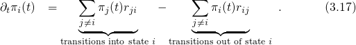
the system can be described by the first-order partial differential equation
The above equation is referred to as the Master or rate equation and controls the
time-dependent occupation probabilities. The first term on the right-hand side
represents the transitions
. The time evolution of
the system can be described by the first-order partial differential equation
The above equation is referred to as the Master or rate equation and controls the
time-dependent occupation probabilities. The first term on the right-hand side
represents the transitions  while the second term stands for the opposite
direction. With the definition
while the second term stands for the opposite
direction. With the definition 
 denotes the matrix belonging to the elements
  . The solution of
equation (3.19) is given by
. The solution of
equation (3.19) is given by 

 vanishes and the equilibrium
occupation probabilities
vanishes and the equilibrium
occupation probabilities  must satisfy
In the case of charge trapping, a single defect is represented by one vector  .
When considering a large ensemble of defects, the stochastic behavior vanishes and
.
When considering a large ensemble of defects, the stochastic behavior vanishes and
 and
and  can be replaced by their corresponding expectation values
 and
and  , respectively. Then the equations (3.19) and (3.22) read
When applying Markov theory to charge trapping in NBTI, each state must be
assigned to a certain configuration and a certain charge state of a defect. The rates
 linking the states
  and
and  must be related to certain defect transitions, such
as charge transfer reactions or thermally activated rearrangements of the defect
structure. The trapping dynamics are then governed by equation (3.23), which must
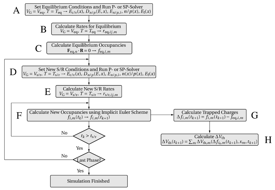
be solved as a function of time. The details of the applied numerical procedures are
outlined in Fig. 3.2.
must be related to certain defect transitions, such
as charge transfer reactions or thermally activated rearrangements of the defect
structure. The trapping dynamics are then governed by equation (3.23), which must
be solved as a function of time. The details of the applied numerical procedures are
outlined in Fig. 3.2.
 ,
,  ) are
calculated in steps A, B, and C. During one stress or relaxation cycle, the band
edges (D) and the transition rates (E) must be determined at first. Then the
corresponding the time-dependent occupations (F) and the resulting threshold
voltage shift (G,F) are evaluated at each time step
) are
calculated in steps A, B, and C. During one stress or relaxation cycle, the band
edges (D) and the transition rates (E) must be determined at first. Then the
corresponding the time-dependent occupations (F) and the resulting threshold
voltage shift (G,F) are evaluated at each time step  . This complete cycle
must be performed for each stress or relaxation phase.
. This complete cycle
must be performed for each stress or relaxation phase.Before the real device is subject to stress, the device is assumed to be in equilibrium.
The corresponding band diagram is computed by a P/SP-solver (A) for the
equilibrium conditions  and
and  . Based on this information, the
transition rates
. Based on this information, the
transition rates  (B) can be evaluated for each defect
  . With the
rates
. With the
rates  at hand, the equilibrium occupation probabilities
  are calculated using the equation (3.24) and must be subsequently stored
(C). When stress sets in, the gate voltage
are calculated using the equation (3.24) and must be subsequently stored
(C). When stress sets in, the gate voltage  and the temperature
  are
changed to
are
changed to  and
and  , respectively. Since this alters the band diagram and
in consequence the transition rates
, respectively. Since this alters the band diagram and
in consequence the transition rates  , the S/SP-solver step (D) and
the calculation of the rates (E) must be repeated. Then the implicit Euler
method is employed for the numerical time integration of equation (3.23).
This iteration scheme must be continued until the end of the stress time
, the S/SP-solver step (D) and
the calculation of the rates (E) must be repeated. Then the implicit Euler
method is employed for the numerical time integration of equation (3.23).
This iteration scheme must be continued until the end of the stress time
 has been reached. At each
  , the change in the defect occupancies
 (G) and the corresponding threshold voltage shift
  (H) are
computed. With the beginning of the relaxation phase,
(H) are
computed. With the beginning of the relaxation phase,  and
and  are
modified again and the whole iteration loop including the steps D, E, F, G, and
H must be repeated. This can be continued for several stress/relaxation
cycles with different stress/relaxation conditions. The steps E, F, and G
of numerical procedure in Fig. 3.2 must be repeated for each individual
defect, where the calculation of the rates requires most of the computation
time.
are
modified again and the whole iteration loop including the steps D, E, F, G, and
H must be repeated. This can be continued for several stress/relaxation
cycles with different stress/relaxation conditions. The steps E, F, and G
of numerical procedure in Fig. 3.2 must be repeated for each individual
defect, where the calculation of the rates requires most of the computation
time.
For the evaluation of  , the charge sheet approximation is employed.
 and
and  are the trap depth and the thickness of the dielectric, respectively. The
above expression gives the threshold voltage shift
are the trap depth and the thickness of the dielectric, respectively. The
above expression gives the threshold voltage shift  due to a single trap
  in
the ‘charged’ state
in
the ‘charged’ state  . It is noted that the term in the parentheses of equation (3.25)
accounts for the trap depth dependence of
. It is noted that the term in the parentheses of equation (3.25)
accounts for the trap depth dependence of  according to which
traps closer to the interface have a larger impact on the threshold voltage.
However, there also exists a strong dependence on the lateral location of the
traps, totally neglected in the above equation. Recall in this context that
the
according to which
traps closer to the interface have a larger impact on the threshold voltage.
However, there also exists a strong dependence on the lateral location of the
traps, totally neglected in the above equation. Recall in this context that
the  steps in the TDDS measurements have also been caused by single
charged traps. The wide variations of these steps have been ascribed to the
position of the traps relative to the current percolation path and follow an
exponential distribution according to an investigation carried out by Kazcer et
al. [50]. This issue has been intensively studied under the name random
dopant fluctuations [132, 133, 134, 50] and gained large interest due to its
serious influence on the lifetime projection. For instance, the charging of one
defect can even produce step heights in the threshold voltage beyond
steps in the TDDS measurements have also been caused by single
charged traps. The wide variations of these steps have been ascribed to the
position of the traps relative to the current percolation path and follow an
exponential distribution according to an investigation carried out by Kazcer et
al. [50]. This issue has been intensively studied under the name random
dopant fluctuations [132, 133, 134, 50] and gained large interest due to its
serious influence on the lifetime projection. For instance, the charging of one
defect can even produce step heights in the threshold voltage beyond  ,
which already violates typical lifetime criteria. By contrast, the charge sheet
approximation rests on the assumption that a trapped charge is distributed over the
whole plane parallel to the interface. Therefore, variations in the threshold
voltage shift due to random dopant fluctuations remain unconsidered in this
approximation.
,
which already violates typical lifetime criteria. By contrast, the charge sheet
approximation rests on the assumption that a trapped charge is distributed over the
whole plane parallel to the interface. Therefore, variations in the threshold
voltage shift due to random dopant fluctuations remain unconsidered in this
approximation.
Small-area devices often contain only a handful of defects. Then the steps B, C, E, F, G, and H can be performed at computationally feasible costs. But since the calculation time increases with the number of defects, the simulation of large-area devices can become time-consuming. In order to reduce computation time for these simulations, a certain number of defects with similar properties are grouped together and replaced by one representative trap. This approach implies that the channel area covers several defects with similar properties including the trap level and the spatial location among others1. Furthermore, it is important to note here that the value of trap density is often quite inaccurate and can differ by some orders of magnitude. Therefore, the number of traps must be treated as a variable in the simulations. This means that the calculated degradation curves can be scaled to the experimental data in order to achieve reasonable agreement of the simulations with the measurements.