So far, only empirical relations, emerging from an experimental perspective but lacking any profound physical justification, have been presented. Now the focus is put on an in-depth microscopic understanding of the NBTI phenomenon. Hence, a series of modeling approaches are discussed in the following, where each of them is traced back to the creation of either interface charges and/or oxide charges.
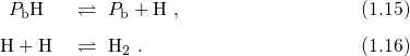
The relation between the threshold voltage shift and the created charges can be expressed as
 being the areal gate capacitance. The change in interface charges
  is given by
  denotes the change in the time-dependent density of interface states at
an energy level
denotes the change in the time-dependent density of interface states at
an energy level  and
and  corresponds to their occupancy. In equation (1.12)
it has been presumed that the temporal charging and discharging of the
interface states are negligible since both processes already occur on much
shorter timescales than that typically covered by NBTI. The interface traps
can hold up to two electrons and exhibit two distinct energy levels, namely
one acceptor and one donor level. Accordingly, they are also referred to as
amphoteric traps [64, 9, 65], which behave as either a donor or an acceptor by
definition (cf. Fig. 1.6). Starting from midgap, a shift of the Fermi level
towards the conduction band charges the interface states negatively, while they
become positively charged if the the Fermi level is moved in the opposite
direction.
corresponds to their occupancy. In equation (1.12)
it has been presumed that the temporal charging and discharging of the
interface states are negligible since both processes already occur on much
shorter timescales than that typically covered by NBTI. The interface traps
can hold up to two electrons and exhibit two distinct energy levels, namely
one acceptor and one donor level. Accordingly, they are also referred to as
amphoteric traps [64, 9, 65], which behave as either a donor or an acceptor by
definition (cf. Fig. 1.6). Starting from midgap, a shift of the Fermi level
towards the conduction band charges the interface states negatively, while they
become positively charged if the the Fermi level is moved in the opposite
direction.
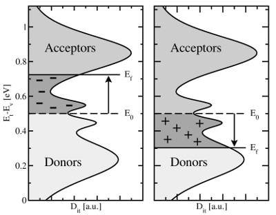
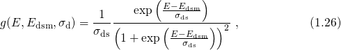
 . Energy levels for
  transitions, termed donor
states, are located below midgap while energy levels for
transitions, termed donor
states, are located below midgap while energy levels for  transitions,
acceptor states, are predominantly found above midgap. The spread of the
peaks in the trap distribution [10, 38] has been speculated to originate from
the disorder of the atomic structure at the interface. Note that in addition to
the interface states density, a band tail states density exponentially decays into
the bandgap. They are ascribed to stretched
transitions,
acceptor states, are predominantly found above midgap. The spread of the
peaks in the trap distribution [10, 38] has been speculated to originate from
the disorder of the atomic structure at the interface. Note that in addition to
the interface states density, a band tail states density exponentially decays into
the bandgap. They are ascribed to stretched  -
- bonds due to the disorder
at the
bonds due to the disorder
at the  interface[66, 67].
In addition to interface charges, also oxide-trapped charges [68, 69, 70] impact the
threshold voltage shift. According to the current understanding of oxide-traps,
charges are stored in preexisting defects whose occupation is governed by the
quantum mechanical trapping dynamics. The contribution of the oxide traps to
 can be evaluated using

 is the density of trap states and
  represents the change in
the trap occupancy. It is commonly assumed that oxide traps have larger time
constants compared to interface states. For instance, this can be related to the depth
of the trap location or the energetical position within the bandgap. Then the
structural disorder of
represents the change in
the trap occupancy. It is commonly assumed that oxide traps have larger time
constants compared to interface states. For instance, this can be related to the depth
of the trap location or the energetical position within the bandgap. Then the
structural disorder of  gives rise to a wide spread of trap levels assumed in
several NBTI models [24].
gives rise to a wide spread of trap levels assumed in
several NBTI models [24].
First serious modeling attempts date back to the so-called reaction-diffusion (RD)
model [71, 72], which has been refined successfully in later studies [25, 68, 73, 74, 60].
It relies on an interface reaction involving the interfacial  dangling bonds (present
in the form of
dangling bonds (present
in the form of  centers) together with some sort of hydrogen species. Initially,
nearly all of the
centers) together with some sort of hydrogen species. Initially,
nearly all of the  centers are supposed to be passivated through a hydrogen
anneal step. This means that their unsaturated
centers are supposed to be passivated through a hydrogen
anneal step. This means that their unsaturated  atoms has established a bond to
a nearby hydrogen atom
atoms has established a bond to
a nearby hydrogen atom  , thereby shifting the electrically active trap levels out of
the substrate bandgap. Upon application of stress, the
, thereby shifting the electrically active trap levels out of
the substrate bandgap. Upon application of stress, the  bonds (
 ) can
break due to the presence of an electric field, thereby activating the forward reaction
of
) can
break due to the presence of an electric field, thereby activating the forward reaction
of
 bonds, the trap levels associated with the
unsaturated
bonds, the trap levels associated with the
unsaturated  atoms are shifted back into the bandgap. Since the released
hydrogen atoms can easily rebond to the
atoms are shifted back into the bandgap. Since the released
hydrogen atoms can easily rebond to the  centers, the reaction (1.14) is in
equilibrium, resulting in a fixed ratio of the concentration of
centers, the reaction (1.14) is in
equilibrium, resulting in a fixed ratio of the concentration of  centers, hydrogen
atoms, and
centers, hydrogen
atoms, and  bonds. The released hydrogen atoms can also diffuse away and
are thus not available for the passivation of the interfacial
bonds. The released hydrogen atoms can also diffuse away and
are thus not available for the passivation of the interfacial  dangling bonds
according to reverse reaction of (1.14). This results in a temporally increasing
concentration of
dangling bonds
according to reverse reaction of (1.14). This results in a temporally increasing
concentration of  centers, measured as a degradation in NBTI. After the removal
of stress, the forward reaction of (1.14) is suppressed while the reverse mode
dominates the reaction dynamics. It is important to note here that the dynamics in
the RD model are eventually governed by the hydrogen diffusion but not by the
interface reaction, which has been assumed to be in equilibrium. An alternative
reaction involves molecular hydrogen
centers, measured as a degradation in NBTI. After the removal
of stress, the forward reaction of (1.14) is suppressed while the reverse mode
dominates the reaction dynamics. It is important to note here that the dynamics in
the RD model are eventually governed by the hydrogen diffusion but not by the
interface reaction, which has been assumed to be in equilibrium. An alternative
reaction involves molecular hydrogen  [75, 76, 77] and presumes that
atomic hydrogen dimerizes instantaneously right at the interface according to
Thus, the generation of interface states is described by the electro-chemical reaction
[75, 76, 77] and presumes that
atomic hydrogen dimerizes instantaneously right at the interface according to
Thus, the generation of interface states is described by the electro-chemical reaction
 and
and  denote the surface concentration of interface states and its initial
concentration, respectively.
denote the surface concentration of interface states and its initial
concentration, respectively.  and
and  stand for the field and temperature
dependent forward and the reverse rate of the interface reaction. The kinetic
exponent
stand for the field and temperature
dependent forward and the reverse rate of the interface reaction. The kinetic
exponent  determines the migrating hydrogen species
  , that is, 1 for atomic
 and
and  , and 2 for molecular
  . Within the RD framework, the interface
reaction (1.17) is assumed to be in equilibrium and thus determines the ratio between
. Within the RD framework, the interface
reaction (1.17) is assumed to be in equilibrium and thus determines the ratio between
 at the interface and
  . However, the basis of the RD model is the transport
equation (1.18) for the migrating species
. However, the basis of the RD model is the transport
equation (1.18) for the migrating species  . It is described by the drift-diffusion
equation which is coupled to the interface reaction via the boundary condition
. It is described by the drift-diffusion
equation which is coupled to the interface reaction via the boundary condition  ,
,  , and
, and  are the diffusion coefficient, the mobility, and the charge
state of the species
are the diffusion coefficient, the mobility, and the charge
state of the species  , respectively. Within the time regime of interest, the
dynamics of the interface reaction are governed by the interfacial hydrogen
concentration, which in turn is controlled by hydrogen diffusion to and from the
interface.
, respectively. Within the time regime of interest, the
dynamics of the interface reaction are governed by the interfacial hydrogen
concentration, which in turn is controlled by hydrogen diffusion to and from the
interface.
A solution of equation (1.17)-(1.19) can be found as

 is referred to as the time exponent. In the case of
  , the RD model
yields a time exponent
, the RD model
yields a time exponent  of
of  , which is only compatible to measurements
obtained with a relatively long delay. In more recent studies with a shorter delay, a
time exponents close to
, which is only compatible to measurements
obtained with a relatively long delay. In more recent studies with a shorter delay, a
time exponents close to  is obtained, as predicted by the RD model for
  .
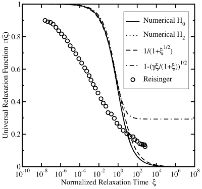
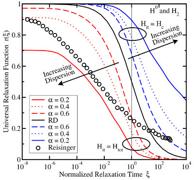
However, thorough examinations of the stress/relaxation curves show large
discrepancies between the RD theory and the universal relaxation (cf. Fig. 1.7).
While the recovery in experiments covers at least 12 decades, the RD model
is limited to about 3 decades. This rules out this model as a reasonable
explanation for NBTI. Some attempts to remedy this deficiency have been put
forward:
.
However, thorough examinations of the stress/relaxation curves show large
discrepancies between the RD theory and the universal relaxation (cf. Fig. 1.7).
While the recovery in experiments covers at least 12 decades, the RD model
is limited to about 3 decades. This rules out this model as a reasonable
explanation for NBTI. Some attempts to remedy this deficiency have been put
forward:
 curves seen in experiments.
 bonds at the gate interface and then migrates inside the poly-gate with a
lower diffusivity. This extension results in a power law with an exponent
of
bonds at the gate interface and then migrates inside the poly-gate with a
lower diffusivity. This extension results in a power law with an exponent
of  during stress but yields a bump during relaxation. As in the case
of the two-region, such a feature has not been observed in experiments.
during stress but yields a bump during relaxation. As in the case
of the two-region, such a feature has not been observed in experiments.
 to
to  for larger stress times
in agreement with some measurements [79, 74]. However, the recovery
remains the same as for the standard RD model and therefore does not
follow the universal relaxation.
for larger stress times
in agreement with some measurements [79, 74]. However, the recovery
remains the same as for the standard RD model and therefore does not
follow the universal relaxation.Experimentally, the most convincing proof that NBTI is not explained by the RD model comes from the TDDS [53, 51]. The spectral maps show clusters which are fixed on the emission time axis for a certain temperature and evolve with increasing stress time. By contrast, the RD model predicts clusters that extend towards larger emission times for rising stress times. Theoretical first-principles calculations of the Pantelides group [80, 81, 82, 83] predict too high dissociation barrier for the interface reactions (1.14) and (1.15-1.16). In contradiction to the assumption of the RD model, Tsetseris et al. [83, 81, 82] proposed that the interface reaction can be initiated by protons originating from the substrate.
In order to explain the long recovery tails seen in experiments, a refinement of the
hydrogen transport in the RD model has been proposed. Due to the exposure to a
hydrogen ambient during device fabrication, a large background concentration of
hydrogen has to be expected. However, this background concentration would strongly
enhance the reverse mode of the interface reaction so that no device degradation
could occur. According to dispersive transport, a large fraction of the hydrogen
particles is bonded to traps and thus cannot participate in the interface reaction.
The retarded release of the strongly bonded particles during recovery [84]
should bring the required long recovery tails. The hydrogen transport has
been modeled to proceed over single trap levels, in which the particles dwell
most of their time. Diffusion only takes place when the hydrogen atoms are
released from their traps. This kind of transport is referred to as dispersive
transport. Its formulation relies on multiple trapping theory [85, 86, 87]
and was combined with the interfacial hydrogen reaction to the reaction
dispersive diffusion (RDD) model [68, 73]. The overall hydrogen  concentration is split into a contribution of free hydrogen
  in a conduction
state and hydrogen
in a conduction
state and hydrogen  residing at traps with an energy level
  :
:
 being the attempt frequency,
  the conduction state for hydrogen, and
 the effective density of conduction states.
  stands for an exponential
trap distribution. Only the free hydrogen as a migrating species
stands for an exponential
trap distribution. Only the free hydrogen as a migrating species  is accounted for
in the diffusion equation: Here, the last term reflects the generation of free hydrogen, which escaped from their
traps. The particular variants of the RDD model primarily differ in the
postulate whether the free hydrogen
is accounted for
in the diffusion equation: Here, the last term reflects the generation of free hydrogen, which escaped from their
traps. The particular variants of the RDD model primarily differ in the
postulate whether the free hydrogen  in the conduction state [88, 25] or the
total hydrogen concentration
in the conduction state [88, 25] or the
total hydrogen concentration  [89, 37] can enter the interface reaction
(1.19). As pointed out in [31], neither variant of the RDD model can explain
the long relaxation tails, irrespective of the assumed hydrogen species (see
Fig. 1.8).
[89, 37] can enter the interface reaction
(1.19). As pointed out in [31], neither variant of the RDD model can explain
the long relaxation tails, irrespective of the assumed hydrogen species (see
Fig. 1.8).
 (red) or
  (blue) for various dispersion parameters
  . In the case of
  the recovery is predicted to end too early while it sets in too late for the
  .
As a consequence, this model is not capable of reproducing the long lasting
relaxation of NBTI.
.
As a consequence, this model is not capable of reproducing the long lasting
relaxation of NBTI.The previous models rest on the assumption that hydrogen diffusion ultimately
governs the generation of interface states. Another modeling approach assumes the
interface reaction as the rate-limiting step. Due to the amorphous structure of  ,
the
,
the  bonds at the interface are subjected to a wide spread of bond lengths
and angles, which are both related to large variations of bond strengths. In order to
account for this fact, the associated dissociation barriers
bonds at the interface are subjected to a wide spread of bond lengths
and angles, which are both related to large variations of bond strengths. In order to
account for this fact, the associated dissociation barriers  [38, 69, 58, 90] are
taken to be distributed rather than single-valued. According to transition state
theory, the bond breakage rates follow an Arrhenius law and can be expressed as
[38, 69, 58, 90] are
taken to be distributed rather than single-valued. According to transition state
theory, the bond breakage rates follow an Arrhenius law and can be expressed as

 is an attempt frequency. Neglecting the corresponding reverse rate,
simple first-order interface kinetics deliver With a Fermi-derivative function for the distributions of dissociation barriers
the interface state generation follows
is an attempt frequency. Neglecting the corresponding reverse rate,
simple first-order interface kinetics deliver With a Fermi-derivative function for the distributions of dissociation barriers
the interface state generation follows 
 , while
the temperature activation originates from the spread
, while
the temperature activation originates from the spread  of the distribution (1.26).
Due to a missing reverse rate
of the distribution (1.26).
Due to a missing reverse rate  , this model cannot explain relaxation
and must thus be assigned to the permanent component of NBTI. In an
improved variant of this model [60], the rate equation (1.25) was extended by a
reverse reaction with distributed barriers. Then the universal relaxation
behavior can be accurately reproduced but the degradation during the stress
phase is drastically underestimated (
, this model cannot explain relaxation
and must thus be assigned to the permanent component of NBTI. In an
improved variant of this model [60], the rate equation (1.25) was extended by a
reverse reaction with distributed barriers. Then the universal relaxation
behavior can be accurately reproduced but the degradation during the stress
phase is drastically underestimated ( ). Therefore, this model falls
short of capturing both the stress and the relaxation phase at the same
time.
). Therefore, this model falls
short of capturing both the stress and the relaxation phase at the same
time.
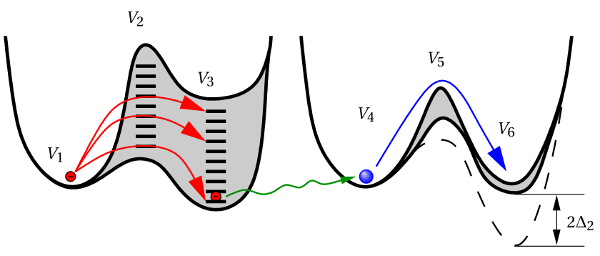
So far, the prolonged degradation and recovery are ascribed to the dispersive nature of either the interface reaction or the hydrogen transport in the oxide. Since both modeling attempts remained fruitless, a new model has been developed, which combines the dispersive interface reaction with a diffusion-like mechanism. The concept of the Born Oppenheimer energy surface [91, 92, 93] motivated the idea of the triple-well model (TWM) [94, 95] where the stable sites of hydrogen along with their separating barriers are represented in one common energy diagram (see Fig. 1.9). The dynamics of this system are expressed by coupled rate equations with Arrhenius-like expressions for transition rates following transition state theory. In a simplified mathematical model, there exist three states corresponding to an equilibrium, an intermediate and a lock-in configuration, which are connected in series. While the temperature activation is already incorporated in Arrhenius-type transition rates, the field acceleration is assumed to be due to an energetical downward shift of the intermediate and the lock-in states along with their connecting barriers (see Fig. 1.9). For instance, this shift can be related to breaking bonds with a dipole moment whose energy contribution depends on the oxide field.
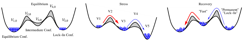
 ,
,  , and
, and  with
the energies
with
the energies  ,
,  , and
, and  ) and their separating barriers (
 and
and
 ). Transitions between two configurations or rather states are indicated
by the arrows. Upon application of stress, the energies
). Transitions between two configurations or rather states are indicated
by the arrows. Upon application of stress, the energies  are shifted down
in energy according to
are shifted down
in energy according to  with
with  being a parameter
and the defects move from state
being a parameter
and the defects move from state  to
to  . When switching back to equilibrium
conditions (recovery), the defects return to the state
. When switching back to equilibrium
conditions (recovery), the defects return to the state  .
.During stress the hydrogen particles travel from the equilibrium towards the lock-in
configuration, where a considerable fraction remains in the intermediate state. After
the stress is removed, particles from the intermediate state first return to the
equilibrium configuration. This fraction of particles correspond to the recoverable
component of NBTI. The return of the other particles from the lock-in configuration
occur at longer timescales and corresponds to the permanent or rather the slowly
recoverable component of NBTI. In  , the first transition mimics the
interface reaction involving the hydrogen atom initially bonded to a
, the first transition mimics the
interface reaction involving the hydrogen atom initially bonded to a  center,
while the lock-in reflects the hydrogen diffusion away from the interface. In
contrast to previous models, the triple-well model cannot only reproduce the
complicated stress/relaxation pattern but also exhibits the correct temperature
activation.
center,
while the lock-in reflects the hydrogen diffusion away from the interface. In
contrast to previous models, the triple-well model cannot only reproduce the
complicated stress/relaxation pattern but also exhibits the correct temperature
activation.
Investigations of the universal recovery (see Section 1.4) have revealed that there
exists a permanent in addition to a recoverable component, where each of them are
caused by their own physical mechanism. As a result, some sort of hole trapping into
defects was suggested as the recoverable component and assumed to be due to elastic
tunneling of holes into preexisting traps [58]. By contrast, a hydrogen reaction like
the  bond breakage in the RD model was ascribed to the permanent
component. However, both mechanisms were assumed to be tightly coupled and
therefore do not take place independently according the argumentation in
Section 1.4.
bond breakage in the RD model was ascribed to the permanent
component. However, both mechanisms were assumed to be tightly coupled and
therefore do not take place independently according the argumentation in
Section 1.4.
A more promising approach assumes hole trapping “triggering” a hydrogen reaction as illustrated in Fig. 1.10. This model [24] relies on thermally activated tunneling into precursor defects. The captured charge weakens the hydrogen bond to the defect and thus causes the release of hydrogen. The last step corresponds to the permanent component of NBTI since the reaction of the defect with hydrogen requires considerably larger times compared to the hole trapping or detrapping process. Even though unprecedented accuracy is achieved for the stress and the relaxation phase at different temperatures and gate voltages, the field dependence of the stress parameter was phenomenologically introduced but has not been justified so far.
 -
- -
- ). The distribution of
  represents the spread
in the hole trap levels, where
represents the spread
in the hole trap levels, where  reflects the required activation energies for
this process. The field acceleration of the hole capture process was modeled by
the term
reflects the required activation energies for
this process. The field acceleration of the hole capture process was modeled by
the term  , where the temperature-independent
  referred to
as the stress parameter. The second step (
referred to
as the stress parameter. The second step ( -
- -
- ) mimics the release of
hydrogen analogously to the description of the TWM.
) mimics the release of
hydrogen analogously to the description of the TWM.