Phenomenological Findings

1.4 Phenomenological Findings

Before embarking on detailed physical models, the focus is now put on a phenomenological understanding of NBTI. In this respect, special attention is put on the functional form of the time evolution of $ΔVth$ depending on gate bias and temperature. Long term extrapolation does not only allow lifetime projection relevant for industrial purposes but also should be viewed as a touchstone for subsequent modeling attempts.

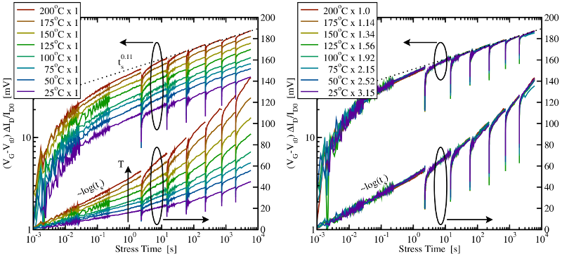
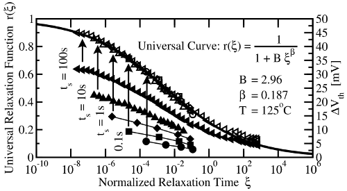
Grasser et al. [24] recognized that the recorded threshold voltage curves follow the same pattern at different stress temperatures and voltages. Therefore, these curves can be scaled so that they overlap for the stress and the relaxation phase. Mathematically, this can be described by

ΔVth(ts,tr,Fox,s,T) = s(T,Fox,s)⋅ΔVt0h(ts,tr). (1.3)

The scaling factor $s(T,Fox,s)$ represents the temperature ( $T$ ) and oxide field ( $Fox,s$ ) dependence, which is best approximated by

s(T,Fox,s) ≈ s0T2F 2ox,s . (1.4)

$ΔV 0th(ts,tr)$ mimics a universally valid shape of the threshold voltage curves. A series of stress sequences for different temperatures are depicted in Fig. 1.3 in order to illustrate the common pattern of the threshold voltage data. As a proof for scalability, all curves line up to one curve by dividing them by their corresponding $s(T,Fox,s)$ . As demonstrated in Fig. 1.3, the initial part of the stress phase shows a logarithmic behavior up to a stress time $ts,0 ~ 1s$ while the subsequent part follows a power-law with an exponent of $n = 0.11$ afterwards. The stress phase [24] can be expressed as

{ ss(T,Fox,s)⋅log10(ts∕t0), ts ≤ ts,0 ΔVth,s(ts,tr,Fox,s,T ) = tns , ts > ts,0 , (1.5)

where $t0$ denotes the first stress measurement point. However, Huard [57] reported that, for some devices, the scalability property is violated for the long term degradation with stress times larger $ts,0 ~ 10s$ . Depending on the details of the fabrication process, the long term part has a scaling factor, which is estimated as

( ) s(T,F ) ≈ sexp - Eact F 4 (1.6) ox,s 0 kBT ox,s

with $Eact$ being an activation energy of $0.15 - 0.25eV$ .

Figure 1.3: Left: The degradation of the drain current recorded for various stress temperatures ( $25 - 200∘C$ ) applying the extended MSM (eMSM) scheme [25, 26]. In this method, the investigated device is subject to exponentially growing stress intervals ( $VG = - 2V$ ) with interruptions of $12s$ (visible as spikes in the plots). During stress, the OTF technique is employed, in which the degradation of threshold voltage is estimated using the expression $ΔVthOTF ≈ (VG - Vth0)(ID - ID0)∕ID0$ . During the short relaxation periods, the drain current is converted to the threshold voltage using a initially recorded $ID(VG)$ curve. Right: The same data as in the left figure, where each curve is multiplied with a suitably chosen factor. All curves share the same shape as proven by the nearly perfect overlap. Note that the degradation lost during the short stress interruptions is restored within less than one decade and thus does not affect the extracted exponent $n$ of the time power-law.

In the context of the universal behavior, special attention has been paid to the recovery phase. This was motivated by the notion that NBTI underlies reversible reaction kinetics. The degradation during the stress phase was assumed to be caused by the combination of a forward and a reverse rate. Therefore, the kinetics during stress were supposed to cover the whole physics, however, the individual contributions of the forward and the reverse rate are obscured. By contrast, only the reverse rate is activated during the relaxation phase, which is thus more suited for analyzing NBTI. In the following, some observations on the relaxation phase are summarized:

The recovery already sets in before the shortest measurable relaxation time of about $1μs$ .
The recovery slows down before reaching the pre-stress level.
The recovery data follow a universal curve when plotted as a function of $ξ = tr∕ts$ .

These observations suggest the following procedure to process the recorded NBTI recovery data: First, the relaxation curves must be normalized to their last respective stress points, which are generally unknown but can be obtained using the back-extrapolation method proposed in [31]. Second, the relaxation times have to be scaled to their last accumulated stress time. The resulting curve can be best analytically described by the empirical relation [31] (cf. Fig. 1.4)

r(ξ) = 1+1Bξβ (1.7)

with $ξ = tr∕ts$ , $B = 0.3- 3$ , and $β = 0.15 - 0.2$ . In a further step, the universal relaxation is extended by the so-called permanent component [58, 28, 26] attributed to a mechanism with another physical origin. This permanent component, however, is ascertained to be a slowly recovering component rather than a constant contribution and is best represented by a power-law [59]. Separating the permanent from the recoverable component $P(ts)$ , the degradation during stress can be written as

ΔVth,s(ts,tr,Fox,s,T) = ss(T, Fox,s) ⋅log10(ts∕t0)+ P (ts) (1.8)

with $t0$ being the first stress measurement point. Alternatively, it can also be formulated as

nr np ΔVth(ts) = Arts + Apts . (1.9)

$Ar∕p$ is the prefactor of a power law with exponent $nr∕p$ , where the subscripts $r$ and $p$ refer to the recoverable or the permanent component, respectively. Note that $np$ is larger than $nr$ in equation (1.9) indicating that the permanent component becomes dominant at large stress times [59]. The impact of the permanent component is demonstrated in Fig. 1.5, where the long term recovery tails deviate from the universal curve. However, universality is regained by accounting for the permanent component. For times longer than $1ms$ , the relaxation data can be well approximated by a logarithmic behavior [60, 61] using the expression

ΔVth,r(ts,tr,Fox,s,T) = sr(T,Fox,s)⋅log10(1+ Cts∕tr)+ P(ts) (1.10)

with $C$ being a parameter. The first term at the right hand side of equation (1.10) represents the recovering component, which shows a nearly logarithmic behavior, and compares well with the short term part of expression (1.7) [60, 31]. In [61] the prefactors $ss(T, Fox,s)$ and $sr(T,Fox,s)$ have been extracted from the eMSM data in Fig. 1.3 for the time range $1ms ...1s$ during stress and $1ms ...100ms$ during relaxation. A comparison of the prefactors has revealed a certain ratio $ss∕sr > 1$ , meaning that the stress and relaxation curves have different slopes. This asymmetry has long remained unrecognized but rules out several proposed NBTI models.

Figure 1.4: Relaxation data measured with the fast MSM technique of Reisinger [27]. Note that all relaxation curves line up to one single curve and thus follow a universal behavior according to equation (1.7) after they have been normalized as indicated by the upwards arrows.

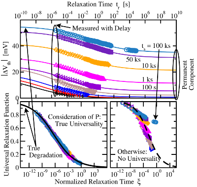
Figure 1.5: MSM data for the relaxation phase [62]. Top: The raw data as a function of $ξ = t ∕t r s$ clearly indicate the existence of a permanent component. Bottom Right: The same as in the top panel but scaled to the last stress value and normalized to the stress time. One can clearly recognize the deviation from the universal behavior $r(ξ)$ . Bottom Left: Only a combination of a recoverable and a permanent component can reproduce the expected universal behavior.

The logarithmic and power-law-like part of the stress curve along with the two components during recovery raise the question whether NBTI is governed by two mechanisms with one of them dominating in each of the time regimes. If this is the case, each of these mechanisms is highly likely to be subject to different field and temperature acceleration. Then the transition between these regimes should be controllable by varying the temperature and the electric field. However, no such transition has been observed so far. In [63], it has been argued that NBTI must be caused by either a single process or two tightly coupled ones. In the latter case, the interplay of both process enforces a single field dependence and temperature dependence without any transitions.

[next] [prev] [prev-tail] [front] [up]