


Next: 3.2.4 Velocity Overshoot
Up: 3.2 Physical Parameters
Previous: 3.2.2 Energy Relaxation Time
3.2.3 Consistent Physical Parameters
The high-field mobility formulas (3.29) and
(3.31) need some further investigation to fully
understand their impact on device modeling. In general the effective
mobilities are defined by
 = q
= q |
(3.35) |
with
 being the momentum relaxation time and m*
 being the
effective carrier mass of the respective carrier. By evaluating the moments
of the distribution functions [29] the momentum relaxation times
can be approximated as functions of the average carrier
energies
w = 3kBT/2 to give (3.31).
being the
effective carrier mass of the respective carrier. By evaluating the moments
of the distribution functions [29] the momentum relaxation times
can be approximated as functions of the average carrier
energies
w = 3kBT/2 to give (3.31).
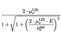
For DD
T = TL is assumed which obviously cannot be used to calculate
the carrier energy and its influence on the mobilities. However, the carrier
temperatures are coupled to the electric field via (3.9) and
(3.10). Assuming a homogeneously doped semiconductor,
divB>S = 0, and the energy balance equations (3.9) and
(3.10) degenerate to the so-called local energy balance equations
which read
Under the assumption of field- and carrier temperature-independent
 equation (3.36) in combination with (3.31)
gives a direct, local dependence of the carrier temperatures and the electric
field
equation (3.36) in combination with (3.31)
gives a direct, local dependence of the carrier temperatures and the electric
field
which can be substituted into (3.31) to find
 (E) (E) |
= |
 |
(3.38) |
which is similar to (3.29) with
 = 2.
However, in (3.29) the driving force
= 2.
However, in (3.29) the driving force
| F |
= |
 grad grad  +
+  . .  . grad . grad  TL . TL . 
  |
(3.39) |
is used instead of the electrical field E. This is done for the following
reasons. (3.38) has been derived under the assumption of a
homogeneous semiconductor. In this case (3.39) reduces to
F =  grad
grad 
 = E which is consistent with the
assumptions given above. On the other hand, (3.38) would
give no velocity saturation for large carrier gradients and low electric
fields. This is obviously unphysical as the carrier velocity for the
resulting diffusion current is limited by the thermal velocity. Equation
(3.38) is very similar to expressions found on a purely
empirical basis. The most common ones are
= E which is consistent with the
assumptions given above. On the other hand, (3.38) would
give no velocity saturation for large carrier gradients and low electric
fields. This is obviously unphysical as the carrier velocity for the
resulting diffusion current is limited by the thermal velocity. Equation
(3.38) is very similar to expressions found on a purely
empirical basis. The most common ones are
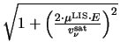
as given by Caughey and Thomas [5] and
as given by Reiser [48]. Both (3.40)
and (3.41) are claimed to perfectly fit measured data
with an appropriate
, normally about
 = 2 for electrons and
 = 1 for holes. For
= 1 both models are equivalent.
= 1 for holes. For
= 1 both models are equivalent.
One problem becomes obvious when comparing
(3.40) and (3.41) with
(3.31). Under homogeneous conditions different mobilities
and hence currents will be obtained for DD and HD simulations except when
using (3.41) with
= 2. This is of
fundamental importance when comparing DD with HD simulations but unfortunately
this problem is generally overlooked in available device simulators.
In general the problem can be stated as follows. In the homogeneous situation
the electric field and the carrier temperatures are related by the local
energy balance equation. The two parameters,  and
and
 have to be
modeled properly to guarantee consistency between the DD and the HD model. In
principle one could start with either
have to be
modeled properly to guarantee consistency between the DD and the HD model. In
principle one could start with either
 (T) or
 (E) to derive the other appropriate model. To derive
(T) from the scattering term of the Boltzmann equation
several assumptions on the distribution function are necessary to get a closed
form solution like (3.31). From a practical point of view
it might seem simpler to start with
(E) as measured data are
more easily available. Nevertheless, as long as closed form solutions exist,
the order is of course irrelevant.
(E) to derive the other appropriate model. To derive
(T) from the scattering term of the Boltzmann equation
several assumptions on the distribution function are necessary to get a closed
form solution like (3.31). From a practical point of view
it might seem simpler to start with
(E) as measured data are
more easily available. Nevertheless, as long as closed form solutions exist,
the order is of course irrelevant.
The following discussion will assume
(E) of the form
| (E) |
= |
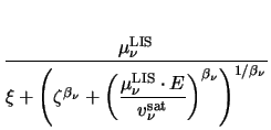 . . |
(3.42) |
Figure 3.1:
Mobility vs. electric field in dependence of the basic parameters
 and
.
and
.
![\begin{figure}
\begin{center}
\resizebox{11.4cm}{!}{
\psfrag{mobGeneral1.0_0.0_1...
...egraphics[width=11.4cm,angle=0]{figures/mobGeneral.eps}}\end{center}\end{figure}](img268.gif) |
With
= 0 and  = 1 one obtains
(3.40), and with
= 1/2 and
= 1/2
(3.41). As these values give the most common expressions,
only
will be used to distinguish between them and an explicit dependence
= 1 one obtains
(3.40), and with
= 1/2 and
= 1/2
(3.41). As these values give the most common expressions,
only
will be used to distinguish between them and an explicit dependence
|
= 1 - |
(3.43) |
will be assumed. It is to note that (3.43) is only used to simplify
reference to the more familiar formulas (3.40)
with
= 0 and (3.41) with
= 1/2.
For these values and
= 1 and
= 2 the mobility
vs. field dependence is shown in Fig. 3.1. In the approach
given above the only assumption made about
was to be independent of
the carrier energy. This approximation is valid for large carrier energies
[16].
In the following the approach outlined above will be generalized starting from
(3.42). Substituting (3.42) in
(3.36) results in
 =
=  |
(3.44) |
which must be solved for
E(T), which is then inserted into
(3.42). The dependence of T vs. E is shown in
Fig. 3.2. Unfortunately (3.44) cannot
be explicitly solved in general. However, it can be solved for the most
important cases
= 0 with arbitrary
and for
= 1/2
with
= 1 or
= 2. After some algebra one obtains
 = 0
= 0 |
: |
*0.0cmE(T) =  . .  a a + + 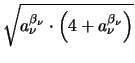
 |
(3.45) |
=  , ,  = 1
= 1 |
: |
E(T) =  . .  a + a + 
 |
(3.46) |
|
= ,
= 2 |
: |
E(T) =   with a = with a =  . .  T T |
(3.47) |
Of course (3.45) with
= 1 is identical
to (3.46) as are the expressions resulting from
(3.42) with the same parameters.
Inserting (3.45), (3.46), and (3.47)
into (3.42) yields
|
= 0 |
: |
 (T) = (T) = 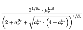 |
(3.48) |
|
= ,
= 1 |
: |
(T) = 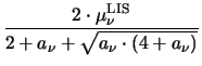 |
(3.49) |
|
= ,
= 2 |
: |
(T) =  |
(3.50) |
A comparison of these mobilities is given in Fig. 3.4. The diffusivity
is defined by the generalized Einstein relation
and is shown in Fig. 3.5. In Fig. 3.5
 = 1/TL has been assumed which gives a 1/T dependence of the mobility
(3.50) and hence a constant diffusivity. This choice
will be justified later.
= 1/TL has been assumed which gives a 1/T dependence of the mobility
(3.50) and hence a constant diffusivity. This choice
will be justified later.
Figure 3.2:
Carrier temperature as a function of electric field for the approach of Hänsch as given by (3.44).
![\begin{figure}
\begin{center}
\resizebox{11.4cm}{!}{
\psfrag{THaensch1.0_0.0_1.0...
...udegraphics[width=11.4cm,angle=0]{figures/THaensch.eps}}\end{center}\end{figure}](img289.gif) |
Figure 3.3:
Carrier temperature as a function of electric field for the approach of Baccarani as given by (3.54).
|
![\resizebox{11.4cm}{!}{
\psfrag{TBacc1.0_0.0_1.0.tbl:y} {$\textstyle \xi = 0,\ \ ...
...(E)\ \ \mathrm{[K]}$}
\includegraphics[width=11.4cm,angle=0]{figures/TBacc.eps}}](img290.gif)
|
A different approach has been proposed by Baccarani and Wordeman [2].
From the generalized Einstein relation it follows that the carrier temperature
can be directly related to the applied field as
They assumed a constant diffusivity
which they justified with experimental data and MC simulation results. However,
(3.53) overestimates
D(E) for large fields [2].
Using (3.52) and (3.53) the carrier
temperature may be expressed as
This dependence is shown in Fig. 3.3. With
(3.42) and (3.54)
E(T) reads
Figure 3.4:
Carrier mobility as a function of carrier temperature for the approach of Hänsch as given by
(3.48)-(3.50).
![\begin{figure}
\begin{center}
\resizebox{11.4cm}{!}{
\psfrag{uHaensch2.0_0.0_1.0...
...udegraphics[width=11.4cm,angle=0]{figures/uHaensch.eps}}\end{center}\end{figure}](img303.gif) |
Figure 3.5:
Carrier diffusion coefficient as a function of carrier temperature for the approach of Hänsch.
|
![\resizebox{11.4cm}{!}{
\psfrag{D1_1.0.crv:y} {$\textstyle \xi = 0,\ \ \beta_{\nu...
...\ \ \mathrm{[K]}$}
\includegraphics[width=11.4cm,angle=0]{figures/DHaensch.eps}}](img304.gif)
|
Figure 3.6:
Carrier energy relaxation time as a function of carrier temperature for the approach of Baccarani.
![\begin{figure}
\begin{center}
\resizebox{11.4cm}{!}{
\psfrag{tauBacc1.0_0.0_1.0....
...ludegraphics[width=11.4cm,angle=0]{figures/tauBacc.eps}}\end{center}\end{figure}](img305.gif) |
From the local energy balance equation the energy relaxation times
may be expressed as
An interesting special case is
= 1/2 and
= 2 in which
(3.42) simplifies to (3.38).
As (3.38) has been derived under the assumption of
an energy independent
one would also expect (3.56)
to result in an energy independent
. This is indeed the case
and one obtains
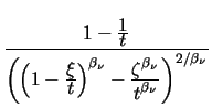
Using (3.57) in (3.50) gives
 = 1/TL and thus
which is in fact (3.54). It is to note that
(3.57) gives a model for
for which both
assumptions produce the same results. However, (3.57)
depends on the low-field mobility which can vary dramatically in the device .
Most unfortunately no measured data could be found as yet in the literature to
confirm this result.
Another interesting feature of (3.56) is
  (T) (T) |
= |
 . .  . .    -
-
 -
- 
 |
(3.59) |
| |
= |
. 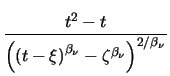 with t = with t = |
(3.60) |
| |
= |
.  |
(3.61) |
| |
= |
|
(3.62) |
independent of
and
> 0 as can also be seen in Fig. 3.6.
With
 = 1400 cm2/Vs and
vsat = 107 cm/s equation
(3.57) gives
= 1400 cm2/Vs and
vsat = 107 cm/s equation
(3.57) gives
 = 0.54 ps. However,
as it is not unrealistic for the low-field mobility to be reduced to 20% of
its maximum value,
is reduced in the very same way.
= 0.54 ps. However,
as it is not unrealistic for the low-field mobility to be reduced to 20% of
its maximum value,
is reduced in the very same way.
Next: 3.2.4 Velocity Overshoot
Up: 3.2 Physical Parameters
Previous: 3.2.2 Energy Relaxation Time
Tibor Grasser
1999-05-31
 - 1
- 1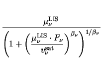


 =
=