The model is based on numerical solution of the time-dependent basic semiconductor equations
where  and
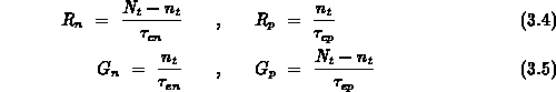
and  are the effective (net) generation rates for electrons and holes, respectively
and
are the effective (net) generation rates for electrons and holes, respectively
and  is the total trapped charge. Our
model allows arbitrary interface and bulk trap distributions in the energy
and position space. Let us consider single-level interface traps with density
is the total trapped charge. Our
model allows arbitrary interface and bulk trap distributions in the energy
and position space. Let us consider single-level interface traps with density
 , located at the position
  along the channel and at the energy
level
along the channel and at the energy
level  . The trap dynamics are described by the
Shockley-Read-Hall equations [409][179]:
. The trap dynamics are described by the
Shockley-Read-Hall equations [409][179]:
where  is the electron recombination rate due to capture of electrons from
the conduction band into traps,
is the electron recombination rate due to capture of electrons from
the conduction band into traps,  the hole recombination rate due to capture
of holes from the valence band (transfer of electrons from traps to the valence
band),
the hole recombination rate due to capture
of holes from the valence band (transfer of electrons from traps to the valence
band),  the electron generation rate due to emission of electrons from
traps to the conduction band and
the electron generation rate due to emission of electrons from
traps to the conduction band and  is the hole generation rate due to
emission of holes from traps (transfer of electrons from the valence band into
traps).
is the hole generation rate due to
emission of holes from traps (transfer of electrons from the valence band into
traps).  is the occupied trap density. The electron and hole capture and
emission time constants are given by
is the occupied trap density. The electron and hole capture and
emission time constants are given by
 ,
,  are the average thermal velocities towards the interface
and
are the average thermal velocities towards the interface
and  ,
,  the average capture cross-sections for electrons and
holes, respectively.
the average capture cross-sections for electrons and
holes, respectively.  ,
,  ,
,  and
and  are effective
density of states and band edge energy for the conduction and valence band,
respectively.
are effective
density of states and band edge energy for the conduction and valence band,
respectively.  and
and  are the electron and hole surface concentrations
at the position . The factor
are the electron and hole surface concentrations
at the position . The factor  , due to trap degeneracy, is assumed
to be unity henceforward
, due to trap degeneracy, is assumed
to be unity henceforward . In the above model,
known as the Shockley-Read-Hall theory, both the conduction and valence band
are reduced to a single energy level with density and energy ,
and , , respectively, whose population is governed by
Maxwell-Boltzmann statistics. Expressions 3.6 represent the
definition for the capture cross-sections which are assumed to be
averaged over the corresponding band ([179]). The
relationships 3.7 follow from the principle of the detailed
balance between both bands and traps, normally holding in equilibrium.
Note that the trap occupancy function
. In the above model,
known as the Shockley-Read-Hall theory, both the conduction and valence band
are reduced to a single energy level with density and energy ,
and , , respectively, whose population is governed by
Maxwell-Boltzmann statistics. Expressions 3.6 represent the
definition for the capture cross-sections which are assumed to be
averaged over the corresponding band ([179]). The
relationships 3.7 follow from the principle of the detailed
balance between both bands and traps, normally holding in equilibrium.
Note that the trap occupancy function  is given in equilibrium
by the Fermi-Dirac statistics
is given in equilibrium
by the Fermi-Dirac statistics
When applying the
relationships 3.4, 3.5, 3.6 and
3.7 to non-equilibrium conditions, it is postulated that
the capture cross-sections associated with the emission and capture processes
remain constant and equal to each other as at the equilibrium - an assumption
neither confirmed nor refuted for interface traps so far. Henceforward, we
also neglect a possible dispersion in values for the capture cross-sections
associated with . Note that our formulation allows arbitrary
dependences of the cross-sections on the energy position and on the local
surface field. In deriving 3.6 and 3.7
Maxwell-Boltzmann statistics are assumed with all carriers at the lattice
temperature. Both conditions are well fulfilled during the course of charge
pumping.
The trap-dynamics equation is given by
where  is the steady-state occupancy function and
  is an
effective time constant which determines the actual trap dynamics
is an
effective time constant which determines the actual trap dynamics
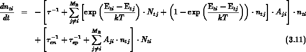
The trap-trap transitions, when more trap levels exist in the forbidden gap,
are not accounted for in equation 3.9 . Such approach
is proper for interface traps. In spite of their possible close location in the
energy space, interface traps are separated in the position space. The electron
wave functions are very localized at the trap site. It is believed, that the
wave functions of neighbour interface traps do not overlap. For bulk traps
trap-trap transitions can take place. Assuming  interacting traps
at the energy levels
interacting traps
at the energy levels  ,
,  , with densities
 and probabilities per unit time
  for the transition of an
electron from level
for the transition of an
electron from level  to level
  , the dynamics
equation for the traps at
, the dynamics
equation for the traps at  becomes
where  denotes the occupied trap density for the level .
The time constants
denotes the occupied trap density for the level .
The time constants  ,
,  and
and  are
the same as defined previously. Dynamics of traps at are
influenced by the dynamics of all trap levels. The system of differential
equations 3.11 (
are
the same as defined previously. Dynamics of traps at are
influenced by the dynamics of all trap levels. The system of differential
equations 3.11 ( ) is of first order and
linear. However, the coefficients of individual equations depend on the solution
of other equations. Since we will consider the interface traps (
) is of first order and
linear. However, the coefficients of individual equations depend on the solution
of other equations. Since we will consider the interface traps ( )
only, all equations 3.11 are independent from each other in our
calculations.
)
only, all equations 3.11 are independent from each other in our
calculations.