So far we have considered the gate pulses with abrupt edges. When the falling
edge  has a nonvanishing width a part of electrons captured at the top
level is emitted at the falling edge before the hole capture occurs. These
electrons are emitted into the conduction band. They are collected by the
junctions and do not contribute to the charge-pumping current. We assume that
the non-steady-state electron emission begins at the gate bias
has a nonvanishing width a part of electrons captured at the top
level is emitted at the falling edge before the hole capture occurs. These
electrons are emitted into the conduction band. They are collected by the
junctions and do not contribute to the charge-pumping current. We assume that
the non-steady-state electron emission begins at the gate bias  and
stops when the hole capture becomes dominant at the gate level
and
stops when the hole capture becomes dominant at the gate level  . The
level specifies the transition between the steady-state and the
non-steady-state emission mode and is given by equaling the rates of changes in
the trap occupancy function in these emission modes, as is explained latter.
has been calculated for different fall times in [97].
It is usually assumed in the literature that the level corresponds
approximately to the device flat-band potential
. The
level specifies the transition between the steady-state and the
non-steady-state emission mode and is given by equaling the rates of changes in
the trap occupancy function in these emission modes, as is explained latter.
has been calculated for different fall times in [97].
It is usually assumed in the literature that the level corresponds
approximately to the device flat-band potential  . In the next section
we will show, when comparing the analytical and the numerical results,
that this assumption is only a very rough approximation. The difference
. In the next section
we will show, when comparing the analytical and the numerical results,
that this assumption is only a very rough approximation. The difference
 remarkably increases with steepness of the gate-pulse
falling edges. In a very rough approximation corresponds to the
device threshold voltage. Note that the levels and
differ from
remarkably increases with steepness of the gate-pulse
falling edges. In a very rough approximation corresponds to the
device threshold voltage. Note that the levels and
differ from  and
and  introduced above.
We adopt a step approximation of the non-steady-state occupancy function
assuming that all traps between  and some emission level
 emit electrons, while the traps bellow the level
do not emit at the falling edge. After [154][97]
emit electrons, while the traps bellow the level
do not emit at the falling edge. After [154][97]
where  is the time of the non-steady-state electron emission and
 is the emission level at the onset of the non-steady-state
emission. This expression can be reduced to
is the emission level at the onset of the non-steady-state
emission. This expression can be reduced to
where  and
and
 is the surface
electron concentration which corresponds to the energy level at the onset of
the non-steady-state emission. The onset level
is the surface
electron concentration which corresponds to the energy level at the onset of
the non-steady-state emission. The onset level  we set to be
When the gate top level is higher than the gate bias which
corresponds to the onset of the non-steady-state emission, the electron emission
occurs in the steady-state mode at first. The non-steady-state mode begins at
the level  , in a step approximation. If the gate top bias
lies below the traps emit immediately in the non-steady-state
mode when the gate bias begins to fall and the onset of the non-steady-state
emission is given by the level .
, in a step approximation. If the gate top bias
lies below the traps emit immediately in the non-steady-state
mode when the gate bias begins to fall and the onset of the non-steady-state
emission is given by the level .
To calculate the level we follow the approach proposed in
the literature [435][434][154][97]. Note that we only judge this
approach as an approximation. Considering the problem
in a rigorous manner, the traps always follow the gate bias with a retardation.
The transition occurs when the splitting between the Fermi level connected with
the current steady-state occupancy function and some ``Fermi level'' associated
with the trap occupancy function exceeds a value of a few  . After this
point the splitting progresses fast in time. This idea to calculate
deserves further investigations.
. After this
point the splitting progresses fast in time. This idea to calculate
deserves further investigations.
Let us assume that the MOS system is in the steady-state conditions before
applying the falling edge of the gate pulse. Note that this assumption is
invalid for short  and low
  , as is discussed at the end of this
section. At the beginning of the falling edge, the change in the total number
of occupied traps occurring in the steady-state emission is given by
, as is discussed at the end of this
section. At the beginning of the falling edge, the change in the total number
of occupied traps occurring in the steady-state emission is given by
where  is the steady-state occupancy function at the current gate bias
 . Considering solely the electron capture and the electron emission
it follows
. Considering solely the electron capture and the electron emission
it follows
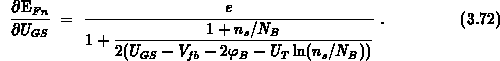
The factor  can be simply calculated by
For a bulk of  -type uniformly doped in a concentration
The term  equals to
  at the falling edge. The function
  ,
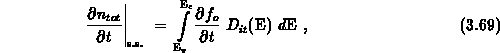
occurring as the subintegral weighting function in 3.69,
reduces to
,
occurring as the subintegral weighting function in 3.69,
reduces to  after a replacement
 . The latter function is peaked at
  and
yields the integral of 1 in the interval
and
yields the integral of 1 in the interval  . Consequently,
expression 3.69 may be approximated by
. Consequently,
expression 3.69 may be approximated by
On the other hand, following [97] we write
in the non-steady-state emission mode which begins at  . Note that
relationship 3.74 is consistent with 3.66.
Equaling expression 3.73 for
. Note that
relationship 3.74 is consistent with 3.66.
Equaling expression 3.73 for
 and
expression 3.74 for we obtain the
transcendental equation
and
expression 3.74 for we obtain the
transcendental equation
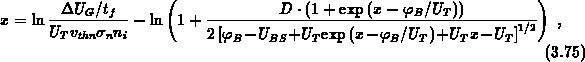
where  and
and
 . This equation is solvable with respect to
 by employing a fixed point linear iteration scheme. The scheme converges
absolutely, since the right-hand-side is a contractive transformation. From the
solution the level follows evidently. The threshold
voltage at the transition point is given by
by employing a fixed point linear iteration scheme. The scheme converges
absolutely, since the right-hand-side is a contractive transformation. From the
solution the level follows evidently. The threshold
voltage at the transition point is given by
where is the solution of 3.75.
According to expression 3.67 the emission level
lies below the level , but close to it if
the emission time  is short and/or
  is long. In the
subthreshold region and for a short , equals to
is long. In the
subthreshold region and for a short , equals to
 . In this case
  and
is close to . In strong inversion,
and
is close to . In strong inversion,
 and
and  hold, the
second term in the brackets at the right-hand-side in 3.66 is
negligible and is independent of
hold, the
second term in the brackets at the right-hand-side in 3.66 is
negligible and is independent of  ,
,  and
and
 . The cases for long and short are more complicated. Then,
 and
and  . It is
expected that splits from . These cases are
not analyzed here.
. It is
expected that splits from . These cases are
not analyzed here.
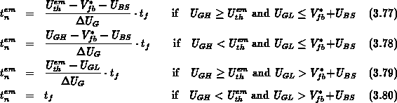
The emission time for electrons at the falling edge of the trapezoidal gate
pulse is approximated by
Note that in the presence of the source-bulk bias  , the level
should be corrected by the back-bias, as is done
in 3.77- 3.80.
, the level
should be corrected by the back-bias, as is done
in 3.77- 3.80.
Accounting for the electron emission at the falling edge, the charge-pumping
current is given by expression 3.63 but with
replaced by .