Next: 3.1 Quasistatische Näherung Up: Dissertation Christian Harlander Previous: 2.2 Erzeugung des Simulationsgitters
In diesem Kapitel werden die physikalischen Zusammenhänge wiedergegeben, die durch partielle Differentialgleichungen und Randbedingungen bestimmt sind. Die Grundlagen der klassischen Elektrodynamik bilden die Maxwell-Gleichungen
Die Materialparameter sind die magnetische Permeabilität ![]() , die
elektrische Permittivität
, die
elektrische Permittivität
![]() , und die elektrische Leitfähigkeit
, und die elektrische Leitfähigkeit
![]() . Die magnetische Permeabilität
. Die magnetische Permeabilität ![]() wird als konstant angenommen,
da keine magnetischen Materialien behandelt werden. Global erfolgen die
Verknüpfungen (3.5, 3.6) über die wesentlich geometrieabhängigen
Kapazitäts- bzw. Induktivitätskoeffizienten.
wird als konstant angenommen,
da keine magnetischen Materialien behandelt werden. Global erfolgen die
Verknüpfungen (3.5, 3.6) über die wesentlich geometrieabhängigen
Kapazitäts- bzw. Induktivitätskoeffizienten.
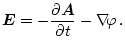
Potenzialformulierungen erweisen sich häufig als günstig, da sie zur Reduktion der Anzahl der Feldvariablen führen. Der Ansatz
Durch die Einführung der Potenziale
![]() ,
, ![]() sind die Felder
sind die Felder
![]() ,
,
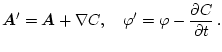
![]() eindeutig festgelegt, allerdings gilt nicht die
Umkehrung, da die Änderung der Potenziale mit einem hinreichend glatten,
beliebigen Skalarfeld
eindeutig festgelegt, allerdings gilt nicht die
Umkehrung, da die Änderung der Potenziale mit einem hinreichend glatten,
beliebigen Skalarfeld ![]() die gleichen Felder
die gleichen Felder
![]() ,
,
![]() ergeben
ergeben
 |
(3.10) |
Zur eindeutigen Festlegung des Vektorpotenzials
![]() ist noch eine Aussage
über die Quellen dieses Feldes zu treffen. Zwei Eichtransformationen haben
sich als besonders vorteilhaft herausgestellt, nämlich die Lorentz-Eichung
und die Coulomb-Eichung.
ist noch eine Aussage
über die Quellen dieses Feldes zu treffen. Zwei Eichtransformationen haben
sich als besonders vorteilhaft herausgestellt, nämlich die Lorentz-Eichung
und die Coulomb-Eichung.
Die Lorentz-Eichung führt zu zwei entkoppelten Wellengleichungen, deren
partikuläre Lösung durch retardierte (verzögerte) Potenziale dargestellt
wird. Dann errechnen sich das Potenzial ![]() und das Vektorpotenzial
und das Vektorpotenzial
![]() nicht aus den derzeitigen Werten, sondern aus
früheren [75,76].
Die Coulomb-Eichung führt auf eine Poisson-Gleichung für das Skalarpotenzial
und für das Vektorpotenzial auf eine Vektor-Poisson-Gleichung, wie
im folgenden Abschnitt gezeigt wird.
nicht aus den derzeitigen Werten, sondern aus
früheren [75,76].
Die Coulomb-Eichung führt auf eine Poisson-Gleichung für das Skalarpotenzial
und für das Vektorpotenzial auf eine Vektor-Poisson-Gleichung, wie
im folgenden Abschnitt gezeigt wird.