7.6 Emission Time Constants
The degraded  in small-area transistors with only a few defects relaxes in
discrete steps. Each step reveals a hole emission event at the emission time
in small-area transistors with only a few defects relaxes in
discrete steps. Each step reveals a hole emission event at the emission time
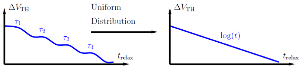
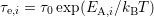 of a particular defect [115, 111]. Larger devices contain
a larger number of defects, which in combination with a nearly uniform
distribution of the activation energies
of a particular defect [115, 111]. Larger devices contain
a larger number of defects, which in combination with a nearly uniform
distribution of the activation energies  yields a log-like recovery behavior as
displayed in Fig. 7.12. As there are many different pairs of
yields a log-like recovery behavior as
displayed in Fig. 7.12. As there are many different pairs of  and
and  within the device, their extraction from the experimental data is discussed
first.
within the device, their extraction from the experimental data is discussed
first.
By subtracting two recovery traces after stress times  and
and  , the
fraction of defects with capture time constants with
, the
fraction of defects with capture time constants with 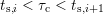 is
determined first [116], which is shown in Fig. 7.13. By dividing the difference
trace into intervals
is
determined first [116], which is shown in Fig. 7.13. By dividing the difference
trace into intervals ![[tr,i,tr,i+1 ]](diss1511x.png) , the fraction of defects having
, the fraction of defects having  and
and  is obtained.
To be able to describe the frequency of occurrence of capture time constants
 and emission time constants
  properly, a large set of long recovery traces
with varying
properly, a large set of long recovery traces
with varying  is needed. The experiments performed cover
  from
from
 up to
up to  and
and  intervals between
  and
and  . This
allows for an extraction of the time constants as exemplarily depicted in
Fig. 7.14.
. This
allows for an extraction of the time constants as exemplarily depicted in
Fig. 7.14.
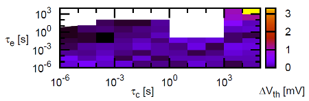
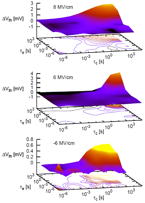
It is now possible to explain the above mentioned effect with the varying
oxide electric field on the basis of Fig. 7.15, where the fraction of  due to
defects with
due to
defects with  and
and  is plotted as smoothed surface over
  and
and
 .
.
For NBTI with an  of
of  the surface shows two peaks.
One peak covers
the surface shows two peaks.
One peak covers  and
and  smaller than
  , while the other more
pronounced one clearly illustrates that the largest part of the degradation was
due to defects with
, while the other more
pronounced one clearly illustrates that the largest part of the degradation was
due to defects with  larger than
  , which is highlighted by the
contour lines below the graph. When comparing the different
, which is highlighted by the
contour lines below the graph. When comparing the different  for
PBTI for
for
PBTI for  covering time constants between
  and
and  , the
peak of
, the
peak of  mainly consists of
  , while it is widened for
 towards smaller
  . This supports the hypothesis of decreased
  for higher
  after PBTI stress, which appears as faster long-term
recovery.
after PBTI stress, which appears as faster long-term
recovery.
 like
in small-area transistors
like
in small-area transistors  behavior, instead.
 and
and  yields the fraction of defects with capture time
constants with
yields the fraction of defects with capture time
constants with  These ranges of capture time constants of
certain defects are depicted as function of
These ranges of capture time constants of
certain defects are depicted as function of  . The contour lines below
the three graphs emphasize the amount of defects contributing to
. The contour lines below
the three graphs emphasize the amount of defects contributing to  .
For NBTI with an
.
For NBTI with an  of
of  , the characteristics of
  are
not changed with increasing
are
not changed with increasing  , despite some shift along the positive
 -axis. The maximum
  values for all
  -ranges are obtained
for small values of
-ranges are obtained
for small values of  . This implies fast relaxation. On the contrary,
PBTI (
. This implies fast relaxation. On the contrary,
PBTI ( ) yields a larger degradation and additionally moves the
characteristics of
) yields a larger degradation and additionally moves the
characteristics of  towards increasing
  . For the largest available
  ,
which covers time constants between
,
which covers time constants between  and
and  , the maximum of
 is moved away from the minimum
  . This maximum marks the
beginning of the change of emission time constants
. This maximum marks the
beginning of the change of emission time constants  depicted in Fig.
  .
. 
 and
and
 is depicted for three different oxide electric fields. The
contour lines below the graphs highlight the biggest changes of
is depicted for three different oxide electric fields. The
contour lines below the graphs highlight the biggest changes of  . Both
surface and contour lines are smoothed for a better visualization. It is shown
that the oxide electric field is related to the magnitude of
. Both
surface and contour lines are smoothed for a better visualization. It is shown
that the oxide electric field is related to the magnitude of  . Increasing
 yields a shift of the peak towards smaller
  , which corresponds to our
monitored increased recovery at larger
, which corresponds to our
monitored increased recovery at larger  . Note that only for
  a
full set of
a
full set of  and
and  is available and therefore the map has to be truncated
in order to be comparable with the case
is available and therefore the map has to be truncated
in order to be comparable with the case  .
.