Measurement Delay

4.2.2 Measurement Delay

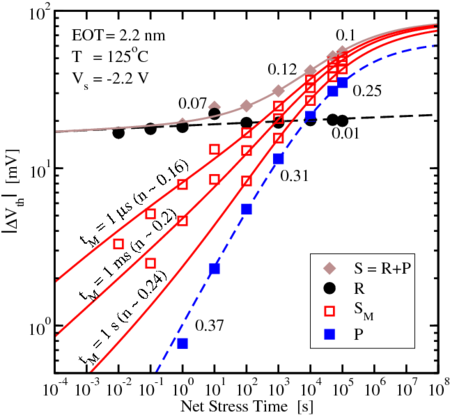
Based on the extracted model parameters of (4.5), a correlation between the observed degradation and the measurement delay can be obtained. The actually observable data marked with $SM$ in Fig. 4.9 is bound between $S = R + P$ (the extrapolated ‘true’ degradation) and $P$ . The larger the delay time, the closer $S M$ and $P$ get and vice versa.

Figure 4.9: Influence of the measurement delay on the observed NBTI behavior (open symbols: data, closed symbols: extracted $R$ and $P$ , lines: model). The measurement results ( $SM$ ) lie between $S$ and $P$ . Depending on the measurement delay of the equipment ( $tM$ ) a broad range of ‘effective’ power-law slopes are observed (limiting values given next to the model lines).

When fitting the single stress sequences with varying $tM$ by a power-law, different values of the slope are obtained which may be a reason why the power-law exponents reported in NBTI literature vary that strongly. In Fig. 4.10 the power-law slopes, defined as $dlog(SM)∕d log(tstr)$ , are shown. As can be seen the extrapolation with a power-law does not seem to be the best choice to represent the time behavior of NBTI due to the interplay between $R$ and $P$ . Since the power-law extrapolation is furthermore only approximately valid over a few decades in time, lifetime prediction based on this approximate concept should be done with great care.

Figure 4.10: Influence of the measurement delay on the observed NBTI behavior (open symbols: data, closed symbols: extracted $R$ and $P$ , lines: model). The effective power-law slope as a function of the measurement delay, defined as $d log (SM )∕d log(tstr)$ is only approximately valid over a few decades in time within the standard measurement window. This is due to the interaction between $R$ (depending on the measurement delay) and $P$ (indepenent of $tM$ ).

[prev] [prev-tail] [front] [up]