
Another possibility to evaluate the kink in the recovery characteristics is to
determine the slope  of the relaxation curve at each point of
 . This is achieved via linear regression using multiple points of
  around
  to obtain the change in its central point
  . Due to the
apparent noise, a multiple-point regression is indispensable; a number of 20, 40,
and 80 data points is used for each
. Due to the
apparent noise, a multiple-point regression is indispensable; a number of 20, 40,
and 80 data points is used for each  . Thereby even very small changes in
 are able to be identified, as illustrated in Fig. 7.11, where the last
relaxation curve of a noisy and a less noisy device is depicted. In this figure the
linear regression performed with 40 data points around each
are able to be identified, as illustrated in Fig. 7.11, where the last
relaxation curve of a noisy and a less noisy device is depicted. In this figure the
linear regression performed with 40 data points around each  yields small
steps where the slope of
yields small
steps where the slope of  suddenly jumps. This issue will be discussed
under the aspect of emission times
suddenly jumps. This issue will be discussed
under the aspect of emission times  of certain defects [111] in the
next section, where changes of the recovery behavior with varying
of certain defects [111] in the
next section, where changes of the recovery behavior with varying  and
and  are due to a change in the emission time rates of the defects
[112, 100, 113, 114, 115].
are due to a change in the emission time rates of the defects
[112, 100, 113, 114, 115].
 identifies even very small changes
in
identifies even very small changes
in  . To suppress the noise multiple points (
 ) are used to
determine the slope
) are used to
determine the slope  via linear regression. This is labeled
by LR
via linear regression. This is labeled
by LR , LR
, LR , and LR
 above. Using linear regression with more
points on the one side smoothes the derivative but on the other hand side
removes information at the beginning and at the end of the
above. Using linear regression with more
points on the one side smoothes the derivative but on the other hand side
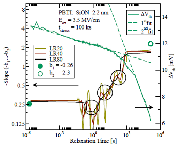
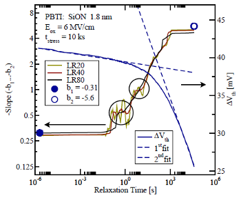
removes information at the beginning and at the end of the  -curve.
This drawback vanishes in the area of interest, around the kink-point.
Left: For noisy data the slope (LR40) suddenly jumps around
-curve.
This drawback vanishes in the area of interest, around the kink-point.
Left: For noisy data the slope (LR40) suddenly jumps around 
 ,
,  , and
, and  , which is marked by circles. Publications dealing
with emission time constants of certain defects provide further information
[100, 113, 111]. Right: For a thinner device the data is less noisy and the
times where the slope changes step-like are more evident, cf.
, which is marked by circles. Publications dealing
with emission time constants of certain defects provide further information
[100, 113, 111]. Right: For a thinner device the data is less noisy and the
times where the slope changes step-like are more evident, cf. 
 and
and  .
.
Note that using even more than 80 data points around each  for the
linear regression would even better suppress the noise but on the other hand side
would disturb important information at the beginning and at the end of the
for the
linear regression would even better suppress the noise but on the other hand side
would disturb important information at the beginning and at the end of the
 -curve. Fortunately, the region of interest (around the kink point) lies in
the center of a
-curve. Fortunately, the region of interest (around the kink point) lies in
the center of a  -curve.