Subsections

• 1.3.1 Order Theory and Sets
• 1.3.2 Cell Topology
• 1.3.3 Complex Topology

1.3 Topological Toolkit

To model space and time within the regime of a finite computer representation, the continuous domain has to be projected onto finite domains or cells. This chapter describes how these cells can be introduced and manipulated algebraically^1.1, and is mainly based on the work of Jänich [2] for common topological terms, Berti [18] for the cell complexes, and Zomorodian [19] for the computational topology part. The most basic property of topology is that it separates global space properties from local geometric attributes. Additionally, and more importantly for this work, it provides a precise notation and language for discussing and handling various properties.

Topological spaces offer several operations for sets and subsets. The formal definition of a topological space is given next, where only the concept of a set is implied:

Definition 3 (Topology)   A topological space $({\ensuremath{X}}, \mathcal{T})$ consists of a set ${\ensuremath{X}}$ and a set $\mathcal{T}$ of subsets, called open sets, of ${\ensuremath{X}}$ such that:

• (T1) $\emptyset \in \mathcal{T}$ and ${\ensuremath{X}} \in \mathcal{T}$.
• (T2) a finite intersection of members of $\mathcal{T}$ is in $\mathcal{T}$.
• (T3) an arbitrary union of members of $\mathcal{T}$ is in $\mathcal{T}$.

The second property (T2) states that arbitrary intersections of subsets have to be in the topological space again. Also the union (T3) of subsets has to be contained in the space. These properties are later used to describe inter-dimensional elements for the complex, such as edges of a cell. An example is given in the following which presents a basic set ${\ensuremath{X}}=\{a,b,c\}$ and the corresponding topology. This pair of the original set and the set of subsets generates the topological space. Vertices are modeled by the singletons $\{a\}$ , $\{b\}$ , and $\{c\}$ .

$$(X, \mathcal{T}) =\{ \emptyset, \{a\},\{b\},\{c\},$$

$$\{a,b\},\{a,c\},\{b,c\},$$

$$\{a,b,c\} \}$$

To handle all subsets in a concise way, the concept of a subspace is introduced.

Definition 4 (Subspaces)   Let $({\ensuremath{X}}, \mathcal{T})$ be a topological space. Any subset ${\ensuremath{Y}}$ of ${\ensuremath{X}}$ inherits a topology in a natural way. It is given by:

$$\mathcal{T}_{\ensuremath{Y}} :={{\ensuremath{V}} \subseteq {\ensu... ... {\ensuremath{Y}} \; \textnormal{for some} \; {\ensuremath{U}} \in \mathcal{T}}$$ (1.23)

To introduce the concept of a topological base, it is necessary to create a topology on a set ${\ensuremath{X}}$ in which a set $\mathcal{S}$ of subsets of ${\ensuremath{X}}$ are open sets.

Definition 5 (Bases)   If $\mathcal{S}$ is already closed under finite intersections, then $\mathcal{T}$ can be defined to be those sets which are unions of sets in $\mathcal{S}$ . Then $\mathcal{T}$ satisfies (T1), (T2), and (T3) and $\mathcal{S}$ is said to be a basis for $\mathcal{T}$ .

In general, to obtain a topology containing $\mathcal{S}$ one has to first form $\mathcal{B}$ , the set of sets which are finite intersections of members of $\mathcal{S}$ , and then define $\mathcal{T}$ to be all arbitrary unions of members of $\mathcal{B}$ . In this case $\mathcal{S}$ is called a sub-basis for $\mathcal{T}$ .

Definition 6 (Homeomorphism)   A homeomorphism ${\ensuremath{f}}: {\ensuremath{X}} \rightarrow {\ensuremath{Y}}$ is a $1-1$ onto function, such that both ${\ensuremath{f}},{\ensuremath{f}}^{-1}$ are continuous.

Then, ${\ensuremath{X}}$ is homeomorphic to ${\ensuremath{Y}}$ , ${\ensuremath{X}} \approx {\ensuremath{Y}}$ . This means that ${\ensuremath{X}}$ and ${\ensuremath{Y}}$ have the same topological type. Homeomorphisms are topological isomorphisms.

With these definitions, sets of subsets can be handled with additional properties in a common way. The common definition for a topological space is very general and allows several topological spaces which are not useful in the field of data structures, e.g., a topological space $({\ensuremath{X}}, \mathcal{T})$ with a trivial topology $\mathcal{T} = \{\emptyset, {\ensuremath{X}}\}$ . Therefore the basic mechanism of separation within a topological space is introduced. Of a hierarchy of possible separation conditions augmenting the topological space axioms, an important characteristic is the Hausdorff condition.

Definition 7 (Hausdorff spaces)   The topological space $(X, \mathcal{T})$ is said to be Hausdorff if, given $x,y \in X$ with $x \ne y$ , there exist open sets $U_1, U_2$ such that $x \in U_1, y \in U_2$ and $U_1 \bigcap U_2 = \emptyset$ .

Common data structures in the field of scientific computing embody the separation characteristics of a Hausdorff space. The assumption to be made is that all scientific data can be modeled by the concept of a Hausdorff space. This can be seen as a generalization of Butler's model, which is based on the assumption that all scientific data can be modeled by trivial fiber bundles [21].

The concept of a cover is introduced to equip a topological space with a type of dimension.

Definition 8 (Cover)   A cover of a set ${\ensuremath{X}}$ is a set of nonempty subsets of ${\ensuremath{X}}$ whose union is ${\ensuremath{X}}$ .

A cover is an open cover if it is contained in the topology.

Definition 9 (Covering Dimension)   A topological space has a (Lebesgue) covering dimension $p$ if any open cover $C$ has a second open cover $D$ , the refinement, where each element $d \in D$ is a subset of an element in the first cover such that no point is included in more than $p+1$ elements.

If a topological space is homeomorphic to $\mathbb{R}^p$ with $p \in \mathbb{N}$ , then its dimension is $p$ . If a space does not have a Lebesgue covering dimension $p$ for any $p \in \mathbb{N}$ , it is called infinite-dimensional. The dimension of the empty set $\emptyset$ is defined as $-1$ . It is important to note that the reverse it not always true, which means that a topological space with dimension $p$ is not necessarily homeomorphic to $\mathbb{R}^p$ .

Another fundamental topological concept is compactness, which may be regarded as a substitute for finiteness. It frequently compensates for the restriction to finite intersections in axiom (T2) by allowing arbitrary sets of open sets to be reduced to finite sets of sets.

Definition 10 (Compactness)   Let $(X, \mathcal{T})$ be a topological space and let $\mathcal{U} := {U_i}_{i \in I} \subseteq \mathcal{T}$ . The set $\mathcal{U}$ is called an open cover of $Y \subseteq X$ if $Y \subseteq \bigcup_{i \in I}$ . A finite subset of $\mathcal{U}$ whose union still contains ${\ensuremath{Y}}$ is a finite sub-cover. It can then be said that ${\ensuremath{Y}}$ is compact if every open cover of ${\ensuremath{Y}}$ has a finite sub-cover.

An important part of the characterization of data structures is the possibility to identify the object with the highest dimension, modeled by the concept of an open cell.

Definition 11 (Open Cell)   A subset $c \subset X$ of a Hausdorff space ${\ensuremath{X}}$ is an open cell if it is homeomorphic to the interior of an open $p$ -dimensional ball $\mathbb{D}^p = \{x \in \mathbb{R}^p : \vert x\vert < 1\}$ .

Collections of cells form larger structures, so-called complexes which are identified by the cell with the highest dimension, e.g., a $p$ -dimensional space contains $p$ -cells.

Definition 12 (Decomposition)   A decomposition $\cal{E}$ of a topological space ${\ensuremath{X}}$ is a decomposition of ${\ensuremath{X}}$ into subspaces.

With the concepts already introduced, the concept of a cell complex can be formulated.

Definition: CW-Complex ${\ensuremath{\mathfrak{K}}}$ [2]
A pair $(\cal{T},E)$ , with $\cal{T}$ a Hausdorff space and a decomposition $\cal{E}$ into cells is called a CW-Complex if and only if the following axioms are satisfied:

• (C1) mapping function: for each $p$ -cell $c \in \cal{E}$ a continuous function $\Phi_e : \mathbb{D}^p \rightarrow \cal{T}$ exists, which transforms $\mathbb{D}^p$ homeomorphically onto the cell $c$ and $\mathbb{S}^{p-1}$ in the union of maximal $(p-1)$ dimensional cells. $\mathbb{D}^p$ represents an $p$ -dimensional closed unit ball and $\mathbb{S}^{p-1}$ represents the sides of $c$ .
• (C2) finite hull: the closed $\mathrm{hull}(c)$ of each cell $c \in \cal{E}$ connects only with a finite number of other cells.
• (C3) weak topology: $A \subset \cal{T}$ is open if and only if each $A \cap \mathrm{hull}(c)$ is open.

A CW-cell complex with the underlying space ${\ensuremath{X}}$ guarantees that all inter-dimensional objects are connected in an appropriate manner, such that $X^{(p)}$ is obtained from $X^{(p-1)}$ by attaching $p$ -cells to each $(p-1)$ -cell and $X^{(-1)}=\emptyset$ . The respective subspaces $X^{(p)}$ are called the $p$ -skeletons of the cell complex.

A $p$ -cell describes the cell with the highest dimension, e.g., $1$ -cell edges and $2$ -cell triangles. For this work the most important property of a CW-complex can be explained by using different $p$ -cells and consistently attaching sub-dimensional cells to the $p$ -cells. This fact is taken care of by the mapping function. For the common case a $p$ -cell can be described by the oriented collection of the 0 -cells, e.g., for a simplex cell $\tau_p = \{v_0, v_1, .., v_p\}, v_i \in {\ensuremath{\mathfrak{K}}}$ , which is introduced in more detail in Section 1.3.1.

So far all mechanisms to handle the underlying topological space of data structures have been introduced. Each subspace can be uniquely characterized by its dimension. All subspaces are connected appropriately by the concept of a finite CW-cell complex.

1.3.1 Order Theory and Sets

The following section introduces concepts of order theory to formalize the combinatorial structure of cells and the global structure of cell complexes [54]. First, the most basic notion of a binary relation is introduced which is a specialization of the relation concept, where two arguments are used.

Definition 13 (Binary relation)   A binary relation $R$ is a subset of the Cartesian product of two sets $A$ and $B$ . That is, any $R \subseteq A \times B$ is a binary relation.

Based on this concept a partial order is defined. A partial order is required to create a hierarchy for our subsets, which can then be used to create our traversal mechanisms.

Definition 14 (Partial order)   A partial order is a binary relation that satisfies the following three properties:

• (PO1) Reflexivity: $a \leq a, \;\; \forall a \in A$ .
• (PO2) Antisymmetry: if $a \leq b$ and $b \leq a \;\;\forall a,b \in A$ , then $a = b$ .
• (PO3) Transitivity: if $a \leq b$ and $b \leq c \;\;\forall a,b,c \in A$ , then $a \leq c$ .

Definition 15 (Partial order on a topological space)   Let $(X, \mathcal{T})$ be a Hausdorff space. For any $x,y \in X$ , a binary relation $\leq$ on ${\ensuremath{X}}$ : $x \leq y$ , if and only if $x \in cl(y)$ is defined, where $cl(y)$ represents the closure for a set within a topological space, where a closure is the intersection of all closed sets containing $y$ . Then this binary relation is a partial order.

Definition 16 (Ordered Sets)   Let $P$ be a set and $\leq$ be a (partial) order on $P$ . Then $P$ and $\leq$ form a (partially) ordered set.

To give examples for ordered sets, Figure 1.2 illustrates the possible terms:

• If the order is total, so that no two elements of $P$ are incomparable, then the ordered set is a totally ordered set, called chain. A formal definition is then given in Section 1.4.

• If no two elements are comparable unless they are equal, then the ordered set is an anti-chain.

• If $P$ has two or more incomparable elements, then the ordered set is a partially ordered set or poset. One example of an incomparable expression is $\{a\}$ with $\{b,c\}$ .

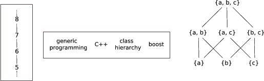
Figure 1.2: Left: Integers form a chain, totally ordered by $\leq$ . Middle: Incomparable items forming an anti-chain. Right: The power-set of $\{a,b,c\}$ ordered by $\leq$ as a partially ordered set.

Definition 17 (Extrema of Partial Ordered Sets [54])   Let $S$ be an ordered set.

• $u \in S$ is said to be maximal in $S$ if and only if there is no $v \in S$ such that $u \leq v$ . A set may have any number of maximal elements, including none.
• If $u$ is $S$ 's only maximal element, then $u$ is the maximum of $S$ .
• The maximum element $u$ (if it exists) is also called the top of $S$ and is denoted by $\top$ .
• Dually, $t \in S$ is said to be minimal in $S$ if and only if there is no $s \in S$ such that $s \leq t$ . A set may have any number of minimal elements, including none.
• If $t$ is $S$ 's only minimal element, then $t$ is the minimum of $S$ .
• The minimum element $t$ (if it exists) is also called the bottom of $S$ and is denoted by $\bot$ .

Finally, the concept of covering is needed. For $x,y \in P$ ordered by $\le$ , it is said $x$ is covered by $y$ (written $x \prec y$ ), if $x < y$ and for any $z \in P$ , $x \le z < y$ implies $x = z$ . This means that there is no element of $P$ "between" $x$ and $y$ . Equivalently it can be said that $y$ covers $x$ .

Definition 18 (Hasse Diagram)   A Hasse diagram of an ordered set is a graph in which:

• Each node corresponds to an element of the set,
• Each edge corresponds to a covering relation between the nodes it connects, and
• If $x$ is covered by $y$ ($x \prec y$ ), then the node for $x$ is drawn in a lower position than the node for $y$ .

It can be seen that in interpreting diagrams, it does not matter whether one node is above or below another unless there is a monotonic path between them; and that if there is a monotonic path from $y$ through one or more nodes down to $x$ , there is no separate edge directly from $y$ to $x$ , as can be seen in Figure 1.2.

Definition 19 (Lattice [18])   A lattice is a bounded poset in which any two elements $a,b$ posses a unique maximal lower bound $\bot$ and a unique minimal upper bound $\top$ .

A lattice, e.g., for $p+1$ -simplices, is atomic, if each element is the $\top$ of elements of dimension $1$ (the atoms), it is coatomic, if each element is the $\bot$ of elements of maximal dimension $p$ (the coatoms).

The $\bot$ of two elements $c_1, c_2$ corresponds to their geometric intersection $\bar c_1 \cap \bar c_2$ , the $\top$ to the element $c$ of least dimension containing both of them $\bar c \subset c_1 \cup c_2$ . The $\top$ of two elements may be the whole mesh. The poset of a convex polytope is an atomic and coatomic lattice. For an arbitrary complex, the poset is in general not a lattice. If a grid's lattice is atomic, it means that $p$ -cells are uniquely determined by their vertex sets if the lattice is coatomic, the vertex sets of $p$ -cells for $p \le n$ can be determined from the knowledge of the vertex sets of the $p$ -cells alone.

1.3.2 Cell Topology

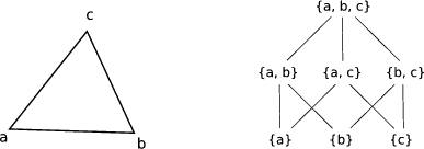
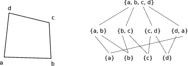
Order concepts for sets just introduced can be used to formalize the internal structure of an arbitrary $p$ -cell, e.g., with the Hasse diagram. A simplex cell is thereby distinguishable from a cuboid cell type in several dimensions as depicted in Figure 1.3 and Figure 1.4, respectively.

Figure 1.3: Cell topology of a simplex cell in two dimensions.

Also, sub-cells such as the corresponding edges and facets and their direct relations to the cell can be identified. An example of extracting all edges of the simplex cell which corresponds with the middle layer of the Hasse diagram can also be seen in Figure 1.3. Another important fact to mention is that the topological structure and the corresponding order hierarchy is invariant of the type of cell used. The $p-1$ -layer of the cuboid cell represents the edges of this type of cell.

Figure 1.4: Cell topology of a cuboid cell in two dimensions.

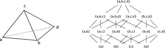
As a higher dimensional example, a three-dimensional simplex example is given in Figure 1.5.

Figure 1.5: Cell topology of a 3-simplex cell.

Here, the $p-1$ -cells are the facets, and, in this particular example, triangles. By using the actual dimension of the $p$ -cell and deriving the $p-n$ cells only by means of the order structure, a flexible framework can be built, where an important property for characterizing cell complexes is required, the regularity of cells and the complex. If the mapping function $\Phi_e$ extends to a homeomorphism on the whole of $\mathbb{D}^p$ , then the $p$ -cell is regular; its sides are then homeomorphic to a decomposition of $\mathbb{S}^{p-1}$ , the boundary. The cell complex ${\ensuremath{\mathfrak{K}}}$ is regular if all cells are regular. The lattice property of a cell complex then guarantees that intersections of the vertex sets of elements always uniquely define a lower dimensional element.

1.3.3 Complex Topology

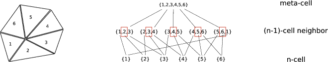
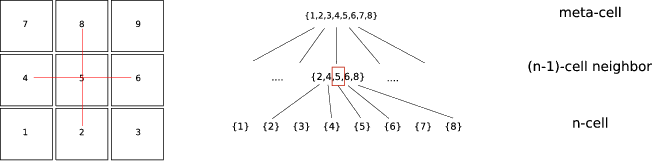
In contrast to the internal cell topology, a cell complex requires adjacence information of cells. There are different possibilities of storing this information efficiently [35,53]. This work develops an abstract means of storing all different types of cells orthogonally, based on the cell topology of the complex topology. For dimensions greater than one, Figure 1.6 illustrates the complex topology of a 2-simplex cell complex where the bottom sets are now the cells. The rectangle in the figure marks the relevant cell number.

Figure 1.6: Complex topology of a simplex cell complex.

The topology of the cell complex is only available locally because of the fact that the top set can have an arbitrary number of elements. The term meta-cell is used to describe various subsets with a common name. In other words, there can be an arbitrary number of triangles in this cell complex attached to the innermost vertex.

Figure 1.7: Complex topology of a cuboid cell complex.

Figure 1.7 presents the complex topology of a cuboid cell complex. The rectangle in the figure marks the main cell (5) under consideration. As can be seen, the number of attached cells is constant inside the space. The topology of the cell complex can thereby be used as a globally known property.

Footnotes

... algebraically^1.1

Appendix A reviews necessary common terms.