8.1 Visual Programming

Based on the concepts of topological manifolds, the separation facilities of the fiber bundle approach, and the correlated programming concepts introduced in Section 4.2, new possibilities for implementing the programming concepts can be derived. One of these concepts is visual programming, which is not only the illustration of a final structure, but can also be used in abstract ways, such as a convergence analysis of non-linear algebraic solver steps, or to define the model by identifying different types of boundary conditions. In addition to a real-time interface to update the visualization at each time step, the following abstract quantities are necessary, such as equation type, coupling coefficients, domain identifier, and boundary conditions. Based on these abstract quantities, the application design can not only be simplified, but the search for errors can also be enhanced by this type of programming.

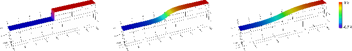
A complete example of an abstract process which greatly benefits from the support of visual programming is given next. Each step of the process of solving a non-linear equation is available to be examined for errors in the implementation. The visualization of the calculation is available in real time, making it possible to observe the evolution even of a non-linear solution process. It proved to be invaluable for the adjustment of simulation parameters. The leftmost part of Figure 8.1 shows the initial potential, while the rightmost depicts the final solution. The center image shows an intermediate result that has not yet fully converged.

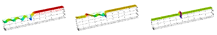
**Figure 8.1:** Potential of a PN diode during different stages of the Newton iteration. From initial (left) to the final result (right).
$\begin{figure}\center \epsfig{figure =figures/application/device/gsse_device_01.eps, angle=0, width=1.0\textwidth}%3.2cm}\end{figure}$

In contrast, an equation system which does not converge is given in Figure 8.2, where small oscillations can be observed. This problem can be caused by wrong input parameters, or by an inappropriate time stepping procedure.

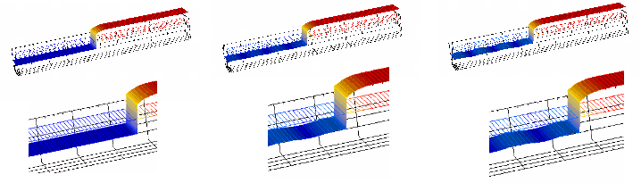**Figure 8.2:** Visualization of non-converging process. Here the potential is illustrated where small oscillations can be observed from left to right.
$\begin{figure}\center \epsfig{figure =figures/rh_diss_visual_nonlinear_01.eps, angle=0, width=1.0\textwidth}%3.2cm}\end{figure}$

Figure 8.3 depicts the complete breakdown of the solution procedure. As can be seen, visual programming greatly supports the development of applications.

**Figure 8.3:** Illustration of a complete breakdown of the solution procedure (from left to right).
$\begin{figure}\center \epsfig{figure =figures/rh_diss_visual_nonlinear_02.eps, angle=0, width=1.0\textwidth}%3.2cm}\end{figure}$