8.2 Wave Equation

An example using the discrete concepts of electromagnetics in conjunction with the comprehensive operations of the GSSEis provided. It translates the continuous formulation of Maxwell's equations given in Section 1.2 with internally oriented $\ensuremath{\mathbf{E}},\ensuremath{\mathbf{B}}$ and externally oriented $\ensuremath{\mathbf{H}},\ensuremath{\mathbf{D}}$ fields, including their linking relations

$$\mathrm{curl} \left( \ensuremath{\mathbf{E}} \right) = -\partial_t \ensuremath{\mathbf{B}}$$ (8.1)

$$\mathrm{curl} \left( \ensuremath{\mathbf{H}} \right) = \partial_t \ensuremath{\mathbf{D}}$$ (8.2)

into a discrete setting, by applying the discrete concepts of chains and cochains (Section 1.4 and Section 1.7). Figure 8.4 presents the discrete form of Faraday's and Amperé's law.

Figure 8.4: The left figure depicts Faraday's law by the corresponding projection onto a finite cell, whereas the right figure illustrates Amperé's law.

Using a projection of the averaged field components onto 2-cells, local representatives of the global quantities are obtained. See Section 2.4.3 for more details. The following equation expresses this fact:

$$\Phi_{B,x\vert(i+1/2,j,k)}^{n+1} = \Phi_{B,x\vert(i+1/2,j,k)}^{n} + \frac{ \Delta x \Delta t }{ \Delta \tilde y \Delta \tilde z }$$ (8.3)

$$( \frac{1}{ \varepsilon_{\vert(i+1/2,j,k+1/2)} } \Psi_{D,x\vert(i+1/2,j,k+1/2)}^{n+1/2} - \frac{1}{ \varepsilon_{\vert(i+1/2,j,k-1/2)} } \Psi_{D,x\vert(i+1/2,j,k-1/2)}^{n+1/2} -$$

$$\frac{1}{ \varepsilon_{\vert(i+1/2,j+1/2,k)} } \Psi_{D,x\vert(i+1/2,j+1/2,k)}^{n+1/2} + \frac{1}{ \varepsilon_{\vert(i+1/2,j-1/2,k)} } \Psi_{D,x\vert(i+1/2,j-1/2,k)}^{n+1/2} )$$

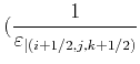
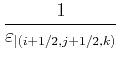
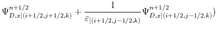
By utilizing the quantity accessor mechanisms and the traversal operations of the GSSE, the equation can be rewritten as a discrete formulation, where the the electric field quantity is located on edges $E_{\mathrm{e}}$ and the magnetic field quantity is located on facets $B_{\mathrm{f}}$ . The permittivity, permeability, and spatial resolution are omitted to emphasize the topological traversal capabilities:

$$\mathcal{L}_\mathrm{B\_fdm} (B)\equiv \frac{ B_{\mathrm{f}}- B^{\... ...t} = \; \Delta_{\mathrm{f}\rightarrow \mathrm{e}} \bigl [ E_\mathrm{e} \bigr ],$$ (8.4)

where ${\mathrm{f}\rightarrow \mathrm{e}}$ denotes the traversal of all edges incident to a face. The topological traversal mechanism is presented in the following code snippet, where the constitutive laws are used to interpolate the corresponding quantities.

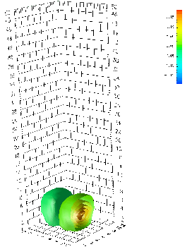
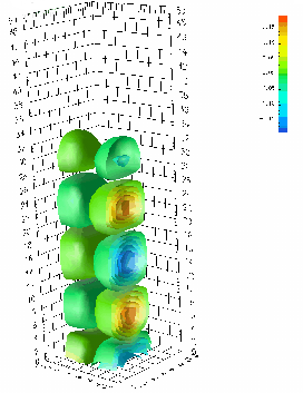
The $x$ -component and $y$ -component of the final vector field $\ensuremath{\mathbf{E}}$ is depicted in Figures 8.5-8.6 for a three-dimensional calculation. The x-y plane with a spatial dimension of $10 \times 10$ units at the bottom uses a simple harmonically oscillating quantity and is also used as a Dirichlet contact. Neumann boundary conditions are applied to the remaining boundary planes.

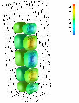
Figure 8.5: Illustration of the $x$ -component of $\ensuremath{\mathbf{E}}$ with a harmonic oscillating source in the x-y plane at two different time steps.

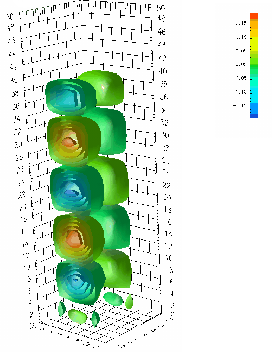
Figure 8.6: Wave equation with a harmonic oscillating source in the x-y plane where the source is switched off. The $y$ -component of $\ensuremath{\mathbf{E}}$ is depicted on the right side.