9.1 Structure Modeling

To overcome the difficulties encountered in the modeling of three-dimensional structures, the Vienna Geometry Modeler (VGM [137]) was developed. It enables an efficient means for structure generation for interconnect simulation, and can be seen as a successor of LAYGRID [114] from the SAP-package. The creation of objects is based on a constructive solid geometry (CSG) approach which models complex three-dimensional shapes using simple objects. The agglomerations of these simple objects then provide suitable simulation structures. To give a brief overview of the syntax and mannerism of VGM, a comparison of a LAYGRID file and a VGM input file are presented next.

First, the LAYGRID input file is presented:

lengthunit { 1.0 um }

mask { MASK0
      rectangle { FX0   SIOX {  0.0  0.0 } { 10.5  6.5 } }
}
mask { MASK1
      rectangle { FX1   SIOX {  0.0  0.0 } { 10.5  6.5 } }
      rectangle { FX2   ALX  {  0.0  2.5 } {  6.0  1.5 } }
      rectangle { FX2C  ALX  {  0.0  2.5 } {  1.0  1.5 } }
}
mask { MASK2
      rectangle { FX3   SIOX {  0.0  0.0 } { 10.5  6.5 } }
      rectangle { FX4   AVX  {  4.6  2.6 } {  0.4  0.4 } }
      rectangle { FX4   AVX  {  5.5  2.6 } {  0.4  0.4 } }
      rectangle { FX4   AVX  {  4.6  3.5 } {  0.4  0.4 } }
      rectangle { FX4   AVX  {  5.5  3.5 } {  0.4  0.4 } }
}
mask { MASK4
      rectangle { FX3   SIOX {  0.0  0.0 } { 10.5  6.5 } }
      rectangle { FX4   AVX  {  4.6  2.6 } {  0.4  0.4 } }
      rectangle { FX4   AVX  {  5.5  2.6 } {  0.4  0.4 } }
      rectangle { FX4   AVX  {  4.6  3.5 } {  0.4  0.4 } }
      rectangle { FX4   AVX  {  5.5  3.5 } {  0.4  0.4 } }
}
mask { MASK5
      rectangle { FX9   SIOX {  0.0  0.0 } { 10.5  6.5 } }
      rectangle { FX10  ALX  {  4.5  2.5 } {  6.0  1.5 } }
      rectangle { FX10C ALX  {  9.5  2.5 } {  1.0  1.5 } }
}
mask { MASK6
      rectangle { FX11  SIOX {  0.0  0.0 } { 10.5  6.5 } }
}
layerstructure {
     origin { 0 0 0 }
     plane { ------------ }
     layer { MASK0    0.5 }
     plane { ------------ }
     layer { MASK1    0.5 }
     plane { ------------ }
     layer { MASK2    0.25 }
     plane { ------------ }
     layer { MASK4    0.25 }
     plane { ------------ }
     layer { MASK5    0.5 }
     plane { ------------ }
     layer { MASK6    0.5 }
     plane { ------------ }
}

Next, the VGM input file is presented:

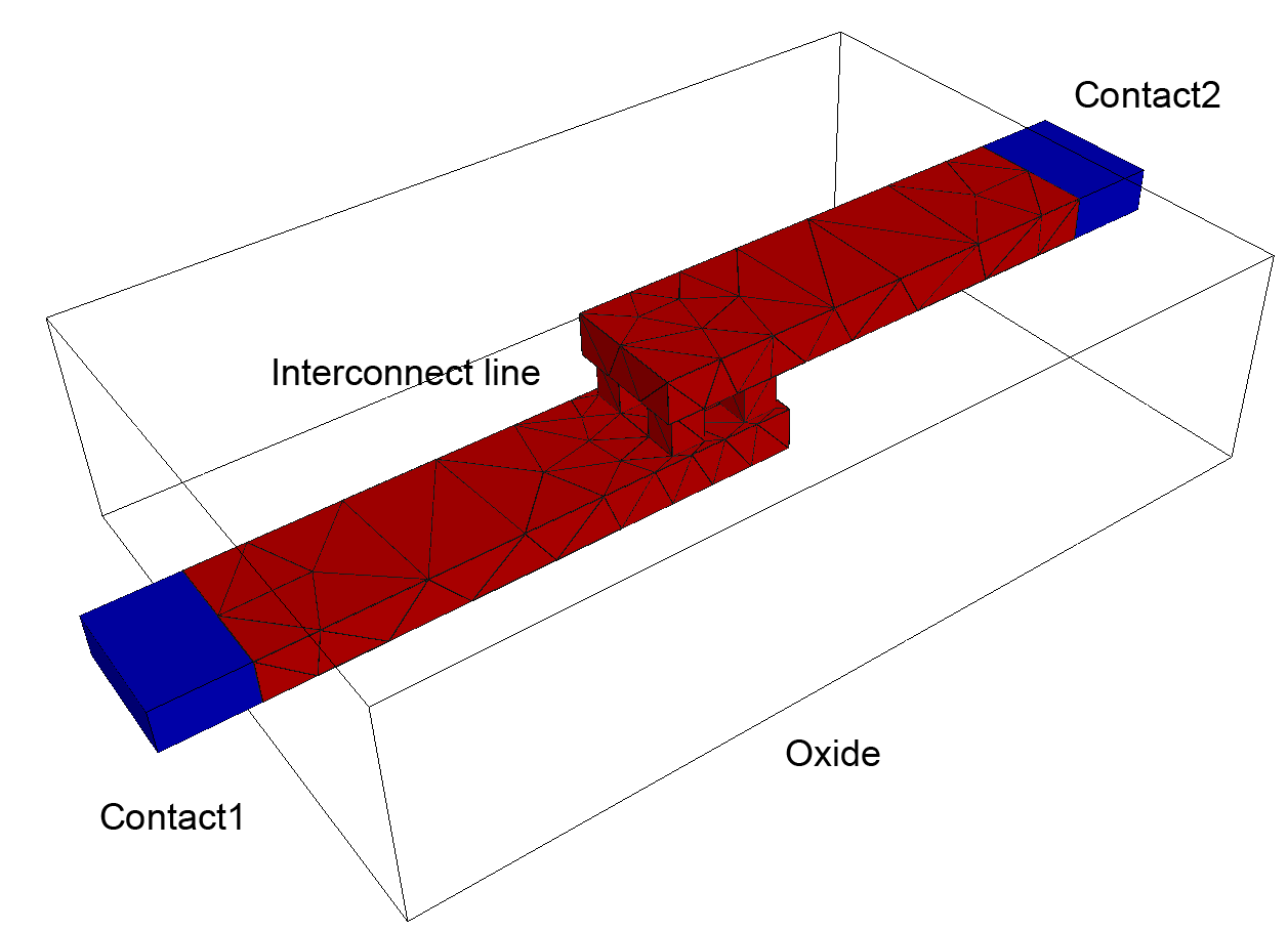
line    { OB  dummy { 0    0  0  }{10  6.5 2.5 } }      
line    { ODL dummy {-10   0  0  }{10  6.5 2.5 } }      
line    { OXR dummy { 10   0  0  }{10  6.5 2.5 } }      
tapered { LB1 dummy {-1   2.5 0.5}{ 7  1.5 0.5}{0.0}{0.0}}
tapered { LB2 dummy { 4.5 2.5 1.5}{6.5 1.5 0.5}{0.0}{0.0}}

tapered { VB1 dummy { 4.6 2.6 0.9}{0.4 0.4 0.7}{0.0}{0.0}}
tapered { VB2 dummy { 5.5 2.6 0.9}{0.4 0.4 0.7}{0.0}{0.0}}
tapered { VB3 dummy { 4.6 3.5 0.9}{0.4 0.4 0.7}{0.0}{0.0}}
tapered { VB4 dummy { 5.5 3.5 0.9}{0.4 0.4 0.7}{0.0}{0.0}}

solid { LT1 dummy { OB & LB1 } }
solid { LT2 dummy { OB & LB2 } }

solid { O1  SiO2 { OB-LB1-LB2-VB1-VB2-VB3-VB4}}
solid { CF1 Al   { ODL & LB1 } }
solid { CF2 Al   { OXR & LB2 } }
solid { LF  Al   { LT1  + LT2 + VB1 + VB2 + VB3 + VB4}}

contact { Contact1   electric 1.0 V {CF1} }
contact { Contact2   electric 0.0 V {CF2} }

Figure 9.1: Resulting structure from the given input specification.

An additional feature of the VGM specification is that tapering angles of the given sidewalls can be easily adjusted. Only the corresponding skewness parameters have to be adjusted, given in the following lines:

//                                                xskew  yskew
  tapered { VB1 dummy { 4.6 2.6 0.9}{0.4 0.4 0.7} {0.0}  {0.0}}

  tapered { VB1 dummy { 4.6 2.6 0.9}{0.4 0.4 0.7} {0.2}  {0.2}}