6.2.4 Scaling of the Ordinary Differential Equation System

A simple scaling yields a more compact form for the ODE system (6.19). An appropriate choice is

 

$$\widetilde{\mathbf{E}}(\mathbf{x})=\mathbf{E}(\mathbf{x}), \quad\... ...(\mathbf{x}),\quad \tilde{\chi}(\mathbf{x}) = \frac{1}{k_0^2} \chi(\mathbf{x}).$$ (6.14)

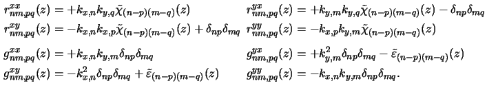
By introducing the Kronecker symbol^b $\delta_{nm}^{}$ the ODEs write to

 

$$\begin{aligned}\frac{d \widetilde{E}_{x,nm}(z)}{d z} &= \sum_{p,q... ...de{E}_{x,pq}(z) + g_{nm,pq}^{yy}(z)\widetilde{E}_{y,pq}(z)\right],\end{aligned}$$

whereby the coefficients are given by

 

$$\begin{alignedat}{2}r_{nm,pq}^{xx}(z) &= +k_{x,n}k_{y,q}\tilde{\c... ...&\;\,g_{nm,pq}^{yy}(z) &= -k_{x,n}k_{y,m}\delta_{np}\delta_{mq}.\end{alignedat}$$

Footnotes

... symbol^b

The Kronecker symbol is defined as $\delta_{nm}^{}$ = 1 for n = m and 0 otherwise.