4.3 Choice of Residual Function

To apply the Newton method a set of variables and a target function has to be specified. A natural choice for the unknowns are the even moments and the potential. Other choices are possible and are discussed in the section on linesearch (see Section 4.4). We did not try to include the odd moments in the set of variables. In hindsight we regard this as a missed opportunity in the one-dimensional case.

The calculation of the residual function always starts with the calculation of the closure for the sixth moment as a function of the lower order moments.

We then have four types of equations: three equations for the moments and one for the potential. The residual vector ${\mathbf{r}}$ is built from the residuals $r_i$ stemming from these four coupled systems.

The choice of residual function is not unique and there are many specifications possible all of which define the same solution. The easiest way is to define the residual as the error from the linear equations 2.74 and the Poisson Equation 2.9.

$$r_i = A_i x_i - y_i \quad \quad i = 1,2,3,4$$ (4.4)

Here $A_i$ is a diffusion operator and $x_i$ stands for $M_2,M_4,$ and $M_6$ and the potential, $y_i$ is the right hand side of the corresponding equation. We call this the linear residual (from ``linear'' quantities $M_0, M_2, M_4,$ and $M_6$).

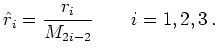
An alternative is to use logarithmic quantities $\log M$ instead of the moments. Rewriting the diffusion equations in these quantities we see that another natural choice for the residual is to use

$$\hat{r}_i = \frac{r_i}{M_{2i}} \quad \quad i = 1,2,3$$ (4.5)

as residual for the moments.

Note that we do not use the logarithmic quantities in the discretization. The linear residual $r_i$ is calculated and then replaced by $\hat{r}_i$. (We mention that in fact we also tried to use logarithmic quantities for the discretization. But this did not result in any improvements.)

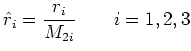
The third variant is similar to the second. Only this time we divide the equation by $M_0, M_2, M_4$ instead of $M_2,M_4,M_6$ and get

$$\hat{r}_i = \frac{r_i}{M_{2i-2}} \quad \quad i = 1,2,3 .$$ (4.6)

Another motivation for variants two and three is, that without it, the residuals from the four types of equations have vastly different orders of magnitude. Even with this form we still have to rescale the residual functions by constant scaling type-dependent factors so that the contribution from each type of equation is approximately of the same order.

Variants two and three can be implemented by reusing the Jacobian $J$ from the first (``linear'') variant. The Jacobian $\hat{J}$ from the modified residual is a simple function of the linear Jacobian $J$.

All the Jacobians are sparse and (depending on the mobility model) can be computed analytically. However, as the formulas become very complex we preferred to use numerical differentiation. With this the only task is the fine-tuning of the step-size for each variant of Jacobian.

We found that the influence on the convergence behavior of the solver is important with respect to performance, and of lesser importance with respect to robustness. Both the second and third variant are superior to the first one and resulted in faster and more uniform convergence. In both respects the third variant seems to be optimal. Hence it pays off to define the residuals in a logarithmic way.