Next: 5.3 Charge Injection Model
Up: 5. Charge Injection Models
Previous: 5.1 Introduction
Subsections
Due to the low mobility in organic semiconductors
 , the diffusion transport is
important for the charge injection process. Therefore, the aim of
this section is to develop an analytical, diffusion-controlled charge
injection model particularly suited for organic light-emitting diodes
(OLED). This model is based on drift-diffusion and multiple trapping
theory. The latter can be used to describe hopping transport in
organic semiconductors [114]. The presented model can explain the
dependence of the injection current on the
temperature, the electric field and the energy barrier height. The
theoretical predictions agree well with experimental data.
The potential barrier
, the diffusion transport is
important for the charge injection process. Therefore, the aim of
this section is to develop an analytical, diffusion-controlled charge
injection model particularly suited for organic light-emitting diodes
(OLED). This model is based on drift-diffusion and multiple trapping
theory. The latter can be used to describe hopping transport in
organic semiconductors [114]. The presented model can explain the
dependence of the injection current on the
temperature, the electric field and the energy barrier height. The
theoretical predictions agree well with experimental data.
The potential barrier
 formed at the metal
semiconductor interface is a superposition of an external electric
field and a Coulomb field binding the carrier on the electrode [115,116],
formed at the metal
semiconductor interface is a superposition of an external electric
field and a Coulomb field binding the carrier on the electrode [115,116],
 |
(5.1) |
Here,  is the distance to the metal-organic layer interface. Since the rapid variation of the
potential 5.1 takes place within
is the distance to the metal-organic layer interface. Since the rapid variation of the
potential 5.1 takes place within  (about 50Å
[117]) in front of the cathode, the field
(about 50Å
[117]) in front of the cathode, the field  can be
regarded as being nearly constant.
can be
regarded as being nearly constant.
Using the drift-diffusion theory, the hole current  can be written as
![$\displaystyle J=-k_BT\mu\left[\frac{q}{k_BT}p_e\left(x\right)\frac{d\varphi\left(x\right)}{dx}+\frac{dp_e\left(x\right)}{dx}\right],$](img444.png) |
(5.2) |
where  is the mobility. On taking and as constant, and solving for
 , we obtain
![$\displaystyle p_e\left(x\right)=\left[N-\frac{J}{k_BT\mu}\int_0^x \exp\left(\fr...
...t)}{k_BT}\right)dx'\right]\exp\left(-\frac{q\varphi\left(x\right)}{k_BT}\right)$](img445.png) |
(5.3) |
where  is
the hole concentration at
is
the hole concentration at  . In multiple trapping
theory [118], the total carrier concentration is given by
a sum of the carrier concentrations in the extended states
. In multiple trapping
theory [118], the total carrier concentration is given by
a sum of the carrier concentrations in the extended states
 and the localized states,
 |
(5.4) |
Here,
 is the density of the localized states,
 is the Fermi Dirac distribution, and the quasi-Fermi energy
  can be written as [118]
where  is the total concentration of localized states,
  is the lifetime of carriers, and
  is the attempt-to-escape
frequency.
is the attempt-to-escape
frequency.
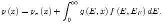
In the injection regime, very close to the contact all the traps are
filled. Moreover, the carrier concentration in the extended states
is much higher than that in the trapped states. At large distance
from the injection contact, the main contribution to the total
carrier concentration comes from the occupied localized states
[112]. So we propose here the concept of a critical
distance , where the carrier concentration in the extended
states equals the carrier concentration in localized states, i.e.,
 |
(5.5) |
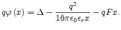
Substituting (5.1),(5.4) and (5.5) into the Poisson equation,
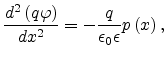 |
(5.6) |
then the critical distance can be calculated as
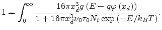 |
(5.7) |
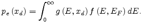
Solving (5.7) with a Gaussian DOS numerically, we can obtain the critical distance
. The free carrier concentration at is calculated by (5.5).
Finally, the injection current can be calculated as
![$\displaystyle J=k_BT\mu\frac{\left[N-p_e\left(x_d\right)\exp\left(\frac{q\varph...
...t)\right]} {\int_0^{x_d}\exp\left(\frac{\varphi\left(x\right)}{k_BT}\right)dx}.$](img455.png) |
(5.8) |
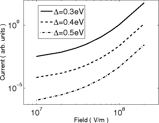
The barrier height  plays an important role for the injection
efficiency. We calculate the relation between the injection current
and the electric field for different , as shown in
Fig 5.1. The parameters are
plays an important role for the injection
efficiency. We calculate the relation between the injection current
and the electric field for different , as shown in
Fig 5.1. The parameters are
 cm
cm ,
,
 eV,
eV,
 s
s ,
,
 s,
s,  K and
K and
 cm
cm /Vs. The
injection current increases with the electric field, and the lower
the , the higher the injection current as intuitively
expected. But the slope of
/Vs. The
injection current increases with the electric field, and the lower
the , the higher the injection current as intuitively
expected. But the slope of  versus
  is not constant.
Figure 5.1:
Dependence of the injection current on the
barrier height.
|
|
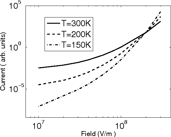
Fig 5.2 shows the temperature dependence of the injection
current for
 , where the other parameters are the same as
in Fig 5.1. The temperature coefficient
decreases strongly with increasing electric field. The coefficient
reverses sign at high electric field, which has also been observed
in [115] theoretically.
, where the other parameters are the same as
in Fig 5.1. The temperature coefficient
decreases strongly with increasing electric field. The coefficient
reverses sign at high electric field, which has also been observed
in [115] theoretically.
Figure 5.2:
Temperature dependencies of the injection current.
|
|
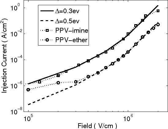
A comparison between the model and experimental data
[112] is shown in Fig 5.3. The
fitting parameters are
 cm,
cm,
 cm/Vs for PPV-ether and
 cm/Vs for PPV-imine, respectively. The
other parameters are the same as in Fig 5.1.
cm/Vs for PPV-imine, respectively. The
other parameters are the same as in Fig 5.1.
Figure 5.3:
Comparison between the model and
experimental data.
|
|
The mobility in organic
materials depends on the local electric field as [119]
 |
(5.9) |
Here  denotes the mobility of carriers at zero field and
 is the parameter describing the field dependence. We first
substitute (5.9) into (5.2) to obtain the carrier concentration,
is the parameter describing the field dependence. We first
substitute (5.9) into (5.2) to obtain the carrier concentration,
![$\displaystyle p_e\left(x\right)=\left[N-\frac{J}{k_BT\mu_0\exp\left(\gamma\sqrt...
...)}{k_BT}\right)dx'\right]\exp\left(-\frac{q\varphi\left(x\right)}{k_BT}\right).$](img473.png) |
(5.10) |
Then, by combining (5.7), (5.10), Gaussian DOS and (5.8), we obtain the injection
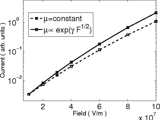
current with the field-dependent mobility. Fig 5.4 illustrates the
relation between injection current and electric field with field
dependent mobility. Parameters are
 cm
cm /Vs,
/Vs,
 (m/V)
(m/V) and
. For
comparison, the injection current with constant mobility is plotted
as well.
and
. For
comparison, the injection current with constant mobility is plotted
as well.
Figure 5.4:
Comparison between injection currents for field dependent mobility
and constant mobility.
|
|
Next: 5.3 Charge Injection Model
Up: 5. Charge Injection Models
Previous: 5.1 Introduction
Ling Li: Charge Transport in Organic Semiconductor Materials and Devices
![$\displaystyle E_F\left(x\right)=k_BT\ln\left[\frac{\nu_0\tau_0N_t}{p_e\left(x\right)}\right],$](img450.png)