5.7 Interface Roughness Scattering

The roughness of interfaces in a heterostructure leads to spatial fluctuations of the well width, and consequently to fluctuations of the energy levels. These fluctuations of the energy levels act as a fluctuating potential for the motion of confined carriers  [89]. A distribution of terraces is present at the interfaces and the electrons are scattered elastically by them  [90].

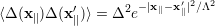
The randomness of the interface is described by a correlation function at the in-plane position x= (x, y), which is usually taken to be Gaussian with a characteristic height of the roughness Δ, and a correlation length Λ representing a length scale for fluctuations of the roughness along the interface  [91], such that

          ′      2 -|x∥-x′∥|2∕Λ2
⟨Δ (x∥)Δ (x ∥)⟩ = Δ  e
(5.32)

The perturbation in the potential V (z) due to a position shift Δ(x) is given by

                                   dV-(z)-
δV  = V[z - Δ(x∥)]- V (z) ≈ - Δ (x∥) dz
(5.33)

For the I-th interface, which is centered about the plane zI and extends over the range [zL,I,zR,I], the scattering matrix element can be defined as
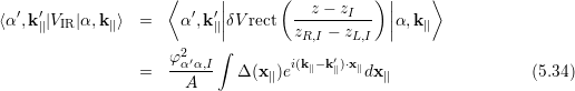
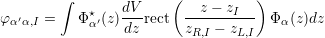
                     ⟨     ||       (  z - zI  ) ||    ⟩
⟨α′,k′∥|VIR |α,k ∥⟩ =    α ′,k′∥||δV rect  ----------  ||α,k∥
                           ∫        zR,I - zL,I
                     φ2α′α,I-         i(k∥-k′∥)⋅x∥
                 =     A     Δ (x∥)e         dx∥                 (5.34)
where |α and |αdenote the final and initial wave functions, respectively. Here, φαα,I is defined as
        ∫        dV     (  z - zI  )
φ α′α,I =   Φ⋆α′(z)---rect ----------  Φ α(z)dz
                 dz      zR,I - zL,I
(5.35)

and the rectangular function reads

         {
rect(z) =   1, |z| ≤ 0.5
            0, |z| > 0.5

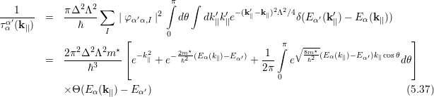
The expectation value of the square of the matrix element is given by

 ′  ′          2   φ2α′α,I∫  ∫     ′         i(k∥- k′)⋅(x∥-x′)  ′
⟨|⟨α ,k ∥|VIR|α,k∥⟩| ⟩ =--A2--     ⟨Δ(x∥)Δ (x∥)⟩e     ∥     ∥ dx∥dx∥
(5.36)

Making use of eq. (5.32) and Fermi’s Golden Rule, the interface roughness induced scattering rates are given by  [92]

                      ∫π   ∫
1 π-Δ2Λ2-∑      ′   2           ′′ - (k′∥-k∥)2Λ2∕4     ′ ′
τα′α(k∥)=    ℏ       | φα α,I |  dθ   dk∥k∥e            δ(Eα (k∥)- E α(k∥))
          I   ⌊       0                                              ⌋
     2 2  2 ⋆     2     2m⋆                ∫π  ∘-8m-⋆
= 2π--Δ-Λ--m- ⌈e- k∥ + e--ℏ2 (Eα(k∥)-E α′) + 1-  e  ℏ2 (Eα (k∥)- Eα′)k∥cosθdθ⌉
       ℏ3                                2π
                                            0
  × Θ(E α(k∥)- E α′)                                                 (5.37)
where k and k are the final and initial wave vectors, respectively, and θ is the scattering angle. The integral is evaluated numerically by means of the MATLAB integration routines.