The density matrix formalism describes the statistical distribution of quantum states in a system [59]. This method allows to treat an ensemble of particles statistically.
Pure States:
The quantum subsystem is described in a Hilbert space of basis functions {Φ1,Φ2,...} and a wave function Ψ represents a generic particle from the ensemble according to
|
| (4.1) |
In the linear combination, the coefficents ci are time dependent and describe the time propagation of the quantum subsystem [60], and
 | (4.2) |
The density operator describes the probability distribution in a system. It takes the form of a projection operator and is defined by
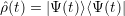 | (4.3) |
The probability of finding a system in state |Φi⟩ is described by the diagonal elements ρii. The degree of coherence is described by the polarization between states |Φi⟩ and |Φj⟩, which is included in the off-diagonal elements ρij. The total population density is conserved, which implies
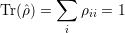 | (4.4) |
The expression for the expectation value of an operator can be written as
![∑ ∑ ⋆ ∑ ∑ ⋆
⟨Ψ |Oˆ|Ψ ⟩ = cicj⟨Φi |Oˆ|Φj ⟩ = cicj ˆOij
i j i j
= ∑ ∑ ρ⋆ ˆO = ∑ ∑ ρ Oˆ
ji ij ij ij
i j i j
= Tr [ρOˆ] (4.5)](diss_html63x.png)
Mixed States:
A mixed state is an incoherent mixture of pure states |Ψ(j)⟩, (j = 1,2,...N) with statistical weights pj which obey [61]
 |
The average value of Ô in the mixed state is given by
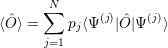 | (4.6) |
The density matrix depends on the pure states involved in the mixed state and their statistical weights according to
 | (4.7) |
The time evolution of the density matrix is obtained by taking the time derivative of the density operator
![∂ρˆ ˆ
iℏ∂t = [ˆρ,H ]](diss_html67x.png) | (4.8) |
with Ĥ = Ĥ 0 + Ĥ′, and Ĥ′ represents a perturbation. This equation of motion is known as the quantum
Liouville equation. Due to the linear transformation of the density operator on the r.h.s in equation
(4.8), it is possible to define a linear operator  which yields
 | (4.9) |
where  denotes the so called Liouville operator
 |
If N is the number of states in the system, the superoperator  is a N2 × N2 matrix and ρ is a N2
dimensional vector. Thus, systems with many states may give rise to insuperable computational
challenges.
is a N2 × N2 matrix and ρ is a N2
dimensional vector. Thus, systems with many states may give rise to insuperable computational
challenges.
We consider a system which is open and in permanent contact with its environment. Under certain conditions the system which is initially in a non-equilibrium state will go over into an equilibrium state after some time. This relaxation process is irreversible.
Let S denote an open quantum system which is coupled to another quantum system R, the environment. The density matrix characterizing the total system is denoted by ρ(t) and the total Hamiltonian by Ĥ = ĤS + ĤR + Ĥ′. In the Schrödinger picture, the equation of motion for the density matrix is given by the Liouville-von Neumann equation
![∂ρ(t) i i ′
-∂t--= -ℏ-[H ˆ0, ρ(t)]- ℏ[ ˆH ,ρ(t)]](diss_html73x.png) | (4.10) |
where Ĥ 0 = Ĥ S + ĤR. Within the interaction picture, the time evolution of the density matrix is controlled only by the interaction Hamiltonian according to
![∂ρI(t) i ′
--∂t--= -ℏ-[H ˆ (t),ρI(t)]](diss_html74x.png) | (4.11) |
Inserting the formal integration
![∫t
i- ′ ˆ′ ′ ′
ρI(t) = ρI(0)- ℏ dt [H (t),ρI(t )]
0](diss_html75x.png) |
into the r.h.s of equation (4.11), the equation of motion for ρI can be expressed as
![∫t
∂-ρI(t) = - i[ ˆH (t),ρ (0)]+-1- dt′[Hˆ′(t),[H ˆ′(t′),ρ (t′)]]
∂t ℏ I ℏ2 I
0](diss_html76x.png) | (4.12) |
The reduced density matrix ρIS which describes the system S is obtained by taking the trace over all variables of system R according to [62]
 | (4.13) |
It is assumed that the interaction starts at t = 0 and that the two systems are uncorrelated prior to this time. Thus
 | (4.14) |
In order to have an irreversible process, it is assumed that R has so many degrees of freedom that it is described by a thermal equlibrium distribution, independent on the amount of energy transferred to it from the system S [63]. Hence
 | (4.15) |
This is the fundamental condition for irreversibility. Using these approximations, the equation of motion for the reduced density matrix can be written as
![∂ρS(t) i 1 ∫t
I = - -TrR [H ˆ′(t),ρS(0)ρR(0)]---2 dt′TrR[ ˆH ′(t),[H ˆ′(t′),ρSI(t′)ρR(0)]]
∂t ℏ ℏ 0](diss_html80x.png) | (4.16) |
According to this equation, the behavior of the system depends on the past events in the time interval [0, t], since the integral contains ρIS(t′). However, the system S is coupled to the reservoir which causes a damping that destroys the ”knowledge” of the past behavior. These considerations lead to the assumption that the system loses all memory of the past. Thus, the substitution
 | (4.17) |
is necessary, which is known as the Markov approximation.
In general, the interaction operator can be expressed as
 | (4.18) |
where  S and
S and  R denote the operators of the dynamic system and the reservoir, respectively. In the
interaction picture we have
R denote the operators of the dynamic system and the reservoir, respectively. In the
interaction picture we have
 | (4.19) |
and
 | (4.20) |
Inserting the interaction operator of this form and the substitution (4.17) into the equation (4.16) and
taking into account that the operators  iS and
  iR commute, yields
 iR(t)⟩ = 0
[64]. The time correlation functions
iR(t)⟩ = 0
[64]. The time correlation functions
 |
describe the average correlation between interactions occuring at times t and t′. The reservoir dissipates quickly the effects of its interaction with the system S. Thus
 |
where τR denotes the correlation time of the reservoir. For t - t′ > τR, interactions become less correlated and the correlation functions satisfy
 |
On the basis of the last considerations we will discuss the Markov approximation. It follows that the integral in equation (4.16) is nonzero only for t′ in the time interval [t - τR,t]. Outside this interval, the values of ρIS(t′) have negligible influence on the time derivative of ρIS(t). The Markov approximation holds if τR is much smaller than a characteristic time that is required for ρIS(t) to change considerably on a macroscopic scale [65].
Since the correlation functions are stationary and depend only on the time difference t′′ = t - t′
 |
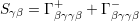
the equation of motion of the reduced density matrix can be written as
![S ∑ ∫∞ (
∂ρI-(t) = - 1-- dt′′ [QˆSi (t),Q ˆSj (t- t′′)ρSI(t)]⟨ˆQRi (t′′)QˆRj ⟩
∂t ℏ2 ij
0 )
- [QˆS (t),ρS (t)QˆS (t- t′′)]⟨ˆQR ˆQR (t′′)⟩ (4.22)
i I j j i](diss_html96x.png)
 |
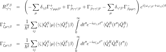
one obtains after some algebra
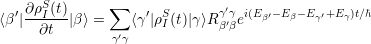 | (4.23) |
where the following abbreviations are used
![′∂ρS(t) i- ′ ˆ S ∑ S ′ S
⟨β|∂t |β⟩ = - ℏ⟨β |[HS, ρ (t)]|β ⟩+ δββ′ ⟨γ|ρ (t)|γ⟩Sβγ - χβ′β⟨β |ρ (t)|β⟩
γ](diss_html100x.png) | (4.24) |
where
 | (4.25) |
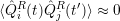
and
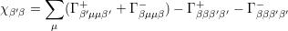 | (4.26) |
Equation (4.24) is called the generalized Master equation and describes the irreversible behavior of a system. In order to get an interpretation of the occuring parameters, we take a look at the rate of change of the diagonal elements of the density matrix. For the diagonal elements, the Schrödinger picture is equivalent to the interaction picture. From the results determined above, it is straightforward to obtain
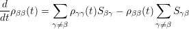 | (4.27) |
This equation is called the Pauli Master equation which plays a fundamental role in modern statistics and can be used in many problems in physics and chemical kinetics [67]. The diagonal elements of the density matrix give the probability of finding the corresponding level occupied at time t. Since the probability increases due to transitions from |γ⟩ to |β⟩, and decreases as a result of transitions from |β⟩ to other states |γ⟩, the parameters Sβγ describe the probability per unit time for the transitions |γ⟩ → |β⟩.
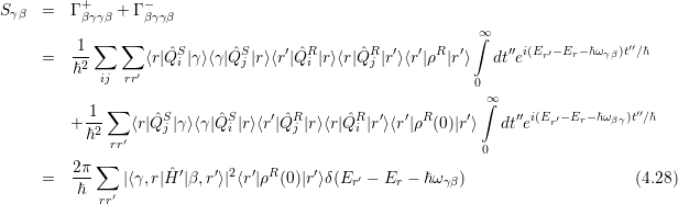
Now we take a more detailed look at the transitions rates. Making use of equation (4.20), the transition rate can be written as
This is the ”Golden Rule” for a transition from level |β⟩ to level |γ⟩. In order to ensure the energy conservation
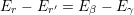 |
the reservoir undergoes simultaneously a transition from a state |r′⟩ to |r⟩. The diagonal elements ⟨r′|ρR(0)|r′⟩ describe the probability of finding the reservoir in a state with energy Er. Reservoirs are in thermal equilibrium. Hence, such a system is represented by an incoherent sum of energy eigenstates with statistical weights1 . Equation (4.27) holds for closed systems. For open systems, a term describing the interaction with the electrical borders has to be added.
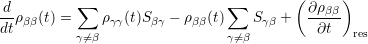 | (4.29) |
The derivation of the Pauli Master equation can be simplified, if the interaction term in equation 4.10 is approximated by a relaxation term
![dρ i ( ∂ρ) ρ- ρeq
---= -[ρ,Hˆ]+ --- - -------
dt ℏ ∂t res τs](diss_html107x.png) | (4.30) |
The last term on the r.h.s expresses the weak interaction with the surroundings. The limit τs →∞ will be taken in the end. Considering the matrix element of the above equation over the eigenstates |α⟩ of the unperturbed Hamiltonian Ĥ0, one gets
![dρββ′= iρ ′(E - E ′ + iℏ ∕τ) + i ∑ [ρ ′′⟨β ′′|Hˆ |β ⟩- ⟨β′|H ˆ |β′′⟩ρ ′′ ′]
dt ℏ ββ β β s ℏ ′′ ′ ββ int int β β
β ⁄=β,β ( )
+ i⟨β|Hˆ |β ′⟩(ρ - ρ ′′)+ -iρ ′[⟨β| ˆH |β⟩- ⟨β ′| ˆH |β′⟩]+ ∂ρ-
ℏ int ββ ββ ℏ ββ int int ∂t res](diss_html108x.png)
![d ρββ i ∑ ′ ′ ( ∂ρ )
--dt- = ℏ- [ρββ′⟨β | ˆHint|β ⟩- ⟨β| ˆHint|β ⟩ρβ′β]+ ∂t-
β′⁄=β res](diss_html109x.png) | (4.31) |
(∂ρ∕∂t)res is assumed to be of order O(αc0), where αc denotes the strength of the interaction Hamiltonian. Equation (4.31) implies that the off diagonal elements of the density matrix are of order O(αc -1 ). To the lowest order, O(αc-1), one can obtain
 |
which implies that ρββ is of the order O(αc-2). Rewriting the last equation as
 |
and inserting into eqaution (4.31), yields
 | (4.32) |
Making use of
 |
one gets for τs →∞
 | (4.33) |
which is formally identical to equation 4.29.
![[ ]
∂ρSI(t) i-∑ ˆS S ˆR R S ˆS ˆR R
∂t=- ℏ Q i (t)ρI(0)TrR (Q i (t)ρ (0))- ρI(0)Q i (t)TrR (Qi (t)ρ (0))
i
1 ∑ ∫t [
- -2- dt′ (ˆQSi (t)QˆSj (t′)ρSI(t)- ˆQSj (t′)ρSI(t)QˆSi (t))TrR (ˆQRi (t)ˆQRj (t′)ρR(0))
ℏ ij 0
]
- (ˆQSi (t)ρSI(t)ˆQSj (t′)- ρSI(t)ˆQSj (t′)QˆSi (t))TrR (ˆQRj (t′)QˆRi (t)ρR(0)) (4.21)](diss_html89x.png)