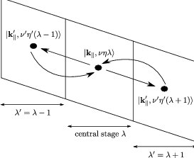
![∑
∂fν+v⋅∇xfν + dp-⋅∇pf ν = {Sν′(k ′,k)fν′(k′)[1- fν(k)]- S ν′(k,k ′)fν(k)[1 - fν′(k ′)]}
∂t dt ′′ ν ν
kν](diss_html115x.png)
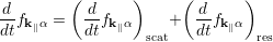
In semiclassical transport theory, electron transport in semiconductor devices is described by the Boltzmann equation given as [68]
|
| (4.34) |
where ν is the subband index. The electron distribution is denoted by the function f(x,p,t) from which the macroscopic quantities of interest can be evaluated. The last two terms on the left hand side (l.h.s) of equation (4.34) describe the net-in flow of electrons to an elementary volume centered at x in position space and at p in momentum space, respectively. The right hand side (r.h.s) represents the collision integral, where the transition rate S(k,k′) from an initial state |k ⟩ to a final state |k′⟩ can be calculated according to the Fermis’s Golden Rule [69]
 | (4.35) |
where Hint denotes the interaction Hamiltonian. In principle, this is the same equation as (4.28) when considering the substitution |α,r⟩→|k⟩. Due to the classical treatment of particles in the l.h.s of the BTE (4.34) and the quantum mechanical one on the r.h.s, the BTE constitutes a semiclassical description. Basically, the semiclassical characterization is based on the assumption that the de Broglie wavelength is significantly smaller than the spatial variation of the external potential. Furthermore, the time between collisions, which is in the range of sub-picoseconds, must be smaller than the time. The collisions are mutually independent and change the electron momentum instantaneously.
In the semiclassical model the transport is described via in- and out-scattering from stationary states that are solutions of the Schrödinger equation. Since the well and barrier structure are included in the Hamiltonian, tunneling is already considered through the eigenstates, and transport occurs via scattering between these states.
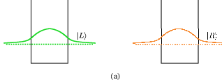
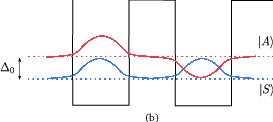
Figure 4.1 illustrates how tunneling between two quantum well states |L⟩ and |R⟩ is described by solving the coupled well system and obtaining a new set of delocalized states. The anticrossing gap Δ0 is the minimum separation between the symmetric and antisymmetric states. Using such delocalized states as basis functions, there is no interwell tunneling time, and intersubband scattering into and out of |A⟩ and |S⟩ from other subbands govern the transport through the barrier. It is shown that this picture is accurate for strong coupling, i.e. large Δ0 [70].
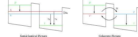
Figure 4.2 shows the difference between the semiclassical and coherent picture of coupled quantum wells. In the semiclassical picture, the wave functions are delocalized at resonance and transport through the barrier happens when electrons enter the levels |S⟩ or |A⟩. In the coherent picture, the electrons are transported through the barrier with Rabi oscillations at frequency Ω.
When the electron dephasing length in the contacts λϕ ~ ℏvth∕δEth is larger than the length of the device L, the electrons are considered to be ”larger” than the device. Here, vth and δEth denote the thermal velocity of the wave packet and the energetic broadening, respectively. In this case, the contacts inject only diagonal elements of the density matrix ρ. Following Van Hove’s observation, the time needed to build the off-diagonal elements of ρ is much longer than the relaxation and transit times [71]. Off-diagonal terms in ρ are built up long after the electron has gone through the device. Thus, a master equation considering only diagonal elements of the density matrix is sufficient to describe electron transport in devices of size L < λϕ [72]. In principle, this picture is equivalent to the Boltzmann description.
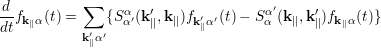
In open systems, the equation describing transport and relaxation phenomena can be written as [73]
 | (4.36) |
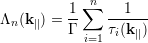
Here, fk ∥α = ρββ, where k∥ is the in-plane wave vector and α ≡ (λ,ν,η) denotes the generic electron state in the multi quantum well structure, i.e. λ is the stage, ν represents the subband index and η stands for the valley index.
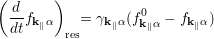
Due to the smallness of the device and the assumption that the electrons are injected as delocalized objects, this approach is practically identical to the approach considered by Fischetti [74]. The second term on the r.h.s of equation (4.36) describes the open boundary conditions of the system. It accounts for the injection and loss contributions from and to external carrier reservoirs treated via a relaxation-time-like term of the form
 | (4.37) |
where γk ∥α-1 is the device transit time of an electron and fk ∥α0 is assumed to be the quasi-equilibrium carrier distribution in the external reservoirs. This assumption is mainly based on the idea that the overall occupations of the ”large” reservoirs of electrons are essentially unchanged by the addition or subtraction of a few electrons to or from the device region.
However, the reservoirs must inject and extract electrons [75]. In the course of solving the Schrödinger equation, a wave incident from outside the device is assumed which is partially reflected and transmitted. It is assumed that outside the device domain a wave is coming from -∞ and is either transmitted to +∞ or it is reflected by the potential and travels back to -∞. The assumption that the wave function is continuous allows to specify the boundary conditions at the contacts. Introducting a reflexion coefficient Rα and transmission coefficient Tα , the total current flowing from the sth contact into other contacts can be written as [74]
 | (4.38) |
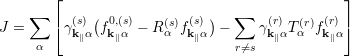
The first term on the r.h.s of equation (4.36) describes the scattering dynamics and is usually treated via collision operators. The master equation can be derived from the Liouville-von Neumann equation using a representation of eigenstates which diagonalize the external potential. The Markov approximation, which ensures the loss of memory effects [76], is the main assumption for the derivation. Fischetti uses additionally the Van Hove limit, which states that αc2t is constant as αc 2 → 0 and the time t tends to infinity, in order to derive the irreversible Pauli master equation and to ensure that the off-diagonal terms of the density matrix remain negligible.
Iotti and coworkers present a somewhat different derivation of the same master equation, calling it Boltzmann-like equation [77]. They also start from the Liouville-von Neumann equation approach and propose the Markov approximation within a fully non-diagonal density matrix treatment. By introducing a so-called diagonal approximation, the off-diagonal elements of the density matrix are neglected arriving finally at the Boltzmann-like or Pauli Master equation
 | (4.39) |
Due to the incoherent nature of the stationary charge transport in QCL heterostructures, the time evolution of the carrier distribution function is governed by the PME (4.39) [78]. Since no electric field is applied in the in-plane direction, the equation (4.39) does not have the in-plane drift and diffusion terms on the l.h.s like in the BTE (4.34). The electrons are not explicitly accelerated along the growth direction, rather the electronic states are affected through the change in the band profile which modifies the electron distribution. Due to scattering the electrons are hopping among the subbands.
Since the QCL structure is translationally invariant, the electron transport can be simulated over a generic central stage only. Due to the small wave function overlap between the central stage and the spatially remote stages, it can be assumed that the interstage scattering is limited only to the nearest neighbor. The electron states corresponding to a single QCL stage are evaluated within a selfconsistent Schrödinger-Poisson solver. Given such carrier states, we consider the multi quantum well structure as a repetition of this periodicity region, which ensures the validity of charge conservation.
The carrier transport is simulated over the central stage and every time a carrier proceeds an interstage scattering process, the electron is reinjected into the central region and the corresponding electron charge contributes to the current. The current density across the device is given in terms of the net electron flux through the interface between the stages
![∑ ∑ (λ+1)ν′η′ ′ (λ-1)ν′η′ ′
J∝ [S λνη (k∥,k∥)fλνη(k ∥)- Sλνη (k ∥,k ∥)fλνη(k∥)]
k∥νηk′∥ν′η′](diss_html125x.png) | (4.40) |
In the Monte Carlo simulation, J is obtained by simply counting the interstage scattering events.
The ensemble Monte Carlo method is an efficient approach for solving the PME (4.39) and simulating electron transport in semiconductor devices in general [79]. It is based on calculating the motion of an ensemble of particles during a short time dt, where electrons are assumed to occupy a known energy state. Electrons can be subject to multiple scattering mechanisms such as electron-longitudinal optical (LO) phonon, acoustic, and optical deformation potential, and intervalley scattering. These scattering mechanisms are considered to be instantaneous and to satisfy transverse momentum conservation and total energy conservation.
Between two consecutive scattering events, which are chosen randomly under consideration of the probability of each scattering mechanism, the electron flies force-free in the in-plane direction and remains in a given subband.
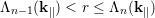
At the end of each free flight a scattering mechanism is selected, where each electron has its own probability of scattering due to its energy and momentum. A scattering mechanism is selected by means of the function Λn defined as
 | (4.41) |
which are the successive summations of the scattering rates normalized with the total scattering rate Γ. By generating a random number r uniformly distributed in the range [0,1], the n-th scattering mechanism is chosen according to [80]
 | (4.42) |
The input for the Monte Carlo transport kernel is provided by a selfconsistent Schrödinger-Poisson solver.
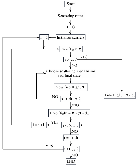
The calculation of the various scattering rates and the algorithm for the determination of the time evolution of the simulated particles are the two major parts of the Monte Carlo simulation. The electrons belonging to one stage are tracked during the simulation. After obtaining the wave functions belonging to the central stage and its neighboring stages, the scattering parameters are calculated. Reinjection of the electrons that scatter out of the central stage ensures the current continuity. Figure 4.4 illustrates the flow chart of the Monte Carlo transport kernel, whose input is provided by the selfconsistent Schrödinger-Poisson solver.
The duration of the free flight τ is determined by random numbers, and the time interval dt is typically chosen to be a few femtoseconds. The number of simulated electrons N and the simulation time ttotal are chosen to allow for reasonable and accurate calculation results, where N = 10000 and ttotal = 10ps are usually sufficient to obtain satisfactory results. Each particle is characterized by a subband index and its in-plane momentum, which are used to determine the available scattering processes. The electron distributions are initialized by randomly assigning the particles to the subbands.
In order to calculate the time evolution of the ensemble of particles, all particles are time-evolved in sequence. Due to the electron dynamics the time interval is chosen small enough (few femtoseconds). During every time step, the initial and the final subbands of the scattered particles are tracked. The current density is obtained from the recorded electron flux due to scattering from the central stage into the next stage or into the previous stage, counting the electrons scattering back as negative. The corresponding charge is weighted by the number of simulated particles. Each simulated particle represents an effective charge
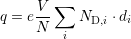 | (4.43) |
where V is the volume of the device, and ND,i represents the donor concentration and di the thickness of the i-th layer.
In general, the ensemble average over the N electrons of the system defines the average value of a
quantity  according to [81]
 | (4.44) |
This average value is compared to previous ones to determine convergence. The number of time steps needed to reach a steady state solution depends on the simulated structure. Usually, the required simulation time accounts for several picoseconds.