Next: E. Diffraction in Far
Up: Dissertation Rainer Minixhofer
Previous: C. General Algorithm for
D. From Boltzmann Distribution to Drift-Diffusion Current Equations
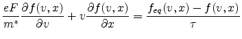
We consider a steady state situation and, for simplicity, a one-dimenstional
geometry [208]. With the use of a relaxation time approximation as in
(3.2) the BOLTZMANN
equation becomes
 |
(D.1) |
Here the relation
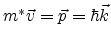 was used, which is valid for a parabolic energy band. Note that the
charge
was used, which is valid for a parabolic energy band. Note that the
charge  has to be taken with the proper sign of the particle
(positive for holes and negative for electrons). A general definition
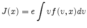
of current density is given by
has to be taken with the proper sign of the particle
(positive for holes and negative for electrons). A general definition
of current density is given by
 |
(D.2) |
where the integral on the right hand side represents the first moment
of the distribution function. This definition of current can be
related to (D.1). After multiplying both sides by  and integrating over v one gets
![$\displaystyle \frac{e F}{m^*} \int v \frac{\partial f(v,x)}{\partial v} dv + \i...
...brace{\int v f_{eq}(v,x) dv}_0 - \int v f(v,x) dv\right] = -\frac{J(x)}{e \tau}$](img467.png) |
(D.3) |
since the function
 is odd in , and its
integral is therefore zero. Thus, one has from (D.3)
is odd in , and its
integral is therefore zero. Thus, one has from (D.3)
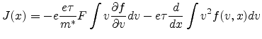 |
(D.4) |
Integrating by parts yields
![$\displaystyle \int v \frac{\partial f}{\partial v} dv = \underbrace{\left[v f(v,x)\right]_{-\infty}^{\infty}}_0 - \int f(v,x) dv = -n(x)$](img470.png) |
(D.5) |
and
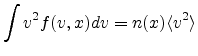 |
(D.6) |
can be written, where
 is the average of the square of the
velocity defined as
is the average of the square of the
velocity defined as
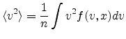 |
(D.7) |
Because of the equipartition theorem, for a purely one-dimensional
treatment, the
 exponent in
(3.3) may be replaced with
exponent in
(3.3) may be replaced with
 ,
while the appropriate thermal kinetic energy becomes
,
while the appropriate thermal kinetic energy becomes
 instead
of
instead
of
 .
.
The drift-diffusion equations are derived introducing the mobility
 and replacing
with
its average equilibrium value
and replacing
with
its average equilibrium value
 , therefore
neglecting thermal effects. The diffusion coefficient
, therefore
neglecting thermal effects. The diffusion coefficient
 (Einstein's relation) is also introduced, and the
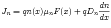
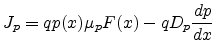
resulting drift-diffusion current is
(Einstein's relation) is also introduced, and the
resulting drift-diffusion current is
where q is used to indicate the absolute value of the electronic
charge. Although no direct assumptions on the non-equilibrium
distribution function  was made in the derivation of
(D.8), the choice of
equilibrium (thermal) velocity means that the drift-diffusion
equations are only valid for very small perturbations of the
equilibrium state (low fields). The validity of the drift-diffusion
equations is empirically extended by introducing
field-dependent mobility
was made in the derivation of
(D.8), the choice of
equilibrium (thermal) velocity means that the drift-diffusion
equations are only valid for very small perturbations of the
equilibrium state (low fields). The validity of the drift-diffusion
equations is empirically extended by introducing
field-dependent mobility  and diffusion coefficient
  ,
obtained from experimental measurements.
,
obtained from experimental measurements.
Next: E. Diffraction in Far
Up: Dissertation Rainer Minixhofer
Previous: C. General Algorithm for
R. Minixhofer: Integrating Technology Simulation
into the Semiconductor Manufacturing Environment