![LDA ∫ 3
EXC [n] = ϵXC(n )n (⃗r)d r.](diss59x.png)
Density functional theory (DFT) is a quantum-mechanical method used in chemistry and physics to calculate the electronic structure of many-body systems, in particular atoms, molecules, and the condensed phases [137,138]. With this theory, the properties of a many-electron system can be determined by using functionals, i.e. functions of another function, which in this case is the spatially dependent electron density. Hence the name density functional theory comes from the use of functionals of the electron density [139]. DFT is among the most popular and versatile methods available in condensed-matter physics, computational physics, and computational chemistry [140].
DFT has been very popular for calculations in solid-state physics since the 1970s [138]. However, DFT was not considered accurate enough for calculations in quantum chemistry until the 1990s, when the approximations used in the theory were greatly refined to better model the exchange and correlation interactions. In many cases the results of DFT calculations for solid-state systems agree quite satisfactorily with experimental data [141,142]. Computational costs are relatively low when compared to traditional methods, such as Hartree-Fock theory and its descendants based on the complex many-electron wave function.
The major problem with DFT is that the exact functionals for exchange and correlation are not known except for the free electron gas. However, approximations exist which permit the calculation of certain physical quantities quite accurately [141]. An approximation to the exchange-correlation term is used. It is called the local density approximation (LDA). For any small region, the exchange-correlation energy is the approximated by that for jellium of the same electron density. In other words, the exchange-correlation hole that is modelled is not the exact one — it is replaced by the hole taken from an electron gas whose density is the same as the local density around the electron [143].
In physics, LDA is the most widely used approximation, where the functional depends only on the density at the coordinate where the functional is evaluated [144]
|
| (3.1) |
The local spin-density approximation (LSDA) is a straightforward generalization of the LDA to include electron spin:
![∫
ELSXDCA [n ↑,n↓] = ϵXC (n↑,n↓)n(⃗r)d3r.](diss60x.png) | (3.2) |
Highly accurate formula for the exchange-correlation energy density ϵXC(n↑,n↓) have been constructed from quantum Monte Carlo simulations of Jellium [145]. Jellium, also known as the uniform electron gas or homogeneous electron gas, is a quantum mechanical model of interacting electrons in a solid where the positive charges (i.e. atomic nuclei) are assumed to be uniformly distributed in space whence the electron density is a uniform quantity as well in space [146].
The interesting point about this approximation is that although the exchange-correlation hole may not be represented well in terms of its shape, the overall effective charge is modelled exactly [146]. This means that the attractive potential which the electron feels at its centre is well described. Not only does the LDA approximation work for materials with slowly varying or homogeneous electron densities but in practise demonstrates surprisingly accurate results for a wide range of ionic, covalent and metallic materials [146].
An alternative, slightly more sophisticated approximation is the generalised gradient approximation (GGA) [147–149] which estimate the contribution of each volume element to the exchange-correlation based upon the magnitude and gradient of the electron density within that element. GGA are still local but also take into account the gradient of the density at the same coordinate:
![∫
EGGXAC [n↑,n↓] = ϵXC (n↑,n ↓, ⃗∇n ↑, ⃗∇n ↓)n(⃗r)d3r.](diss61x.png) | (3.3) |
Using GGA very good results for molecular geometries and ground-state energies have been achieved.
In this work, the imaginary part of the dielectric function is calculated by DFT to investigate the optical properties of studied structures [150]. If the incident light is assumed to be polarized along the transport direction (x-axis), the imaginary part of the dielectric function in the linear response regime is given by [150]
| εi(ω) = |   2 ∑
kx|pc,v|2δ 2 ∑
kx|pc,v|2δ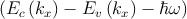 | ||
×![[f (Ev (kx)) - f (Ec (kx))]](diss65x.png) , , | (3.4) |
The summation in Eq. 3.4 can be converted into an energy integration by introducing the joint density of states (JDOS) defined as
 | (3.5) |
where Skx is the constant energy surface defined by Ec - Ev
- Ev = ℏω.
= ℏω.
The real part of the dielectric function εr(ω) can be evaluated from the imaginary part using the Kramers-Kronig relation [150]. The interband dielectric function is related to the optical conductivity by ε(ω) = 1 + 4πiσ(ω)∕ω [151].
For DFT calculations, we employed the Spanish Initiative for Electronic
Simulations with Thousands of Atoms (SIESTA) package [152] with the
following parameters: double-ζ basis set with additional orbitals of polarization
for total energies and electronic band-structures calculations, the generalized
gradient approximation method, Perdew-Burke-Ernzerhof (PBE) as the
exchange-correlation function, and the Troullier-Martins scheme for the
norm-conserving pseudopotential calculations [135]. A grid cutoff of 210 Ry is
used and the Brillouin zone sampling is performed by the Monkhost pack mesh of
k-points. A mesh of  has been adopted for discretization of k-points
and a broadening factor of 0.1eV is assumed for the joint density of states
calculation, and the convergence criterion for the density matrix is taken as
10-4.
has been adopted for discretization of k-points
and a broadening factor of 0.1eV is assumed for the joint density of states
calculation, and the convergence criterion for the density matrix is taken as
10-4.
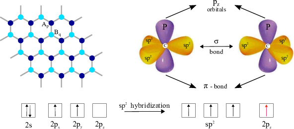
In graphene three σ bonds hybridize in an sp2 configuration, whereas the other 2pz orbital, which is perpendicular to the graphene layer, forms π covalent bonds. Each atom in an sp2-coordination has three nearest neighbors, located acc = 1.42 Å away, see Fig. 3.1. It is well known that the electronic and optical properties of GNRs are mainly determined by the π electrons [153]. To model these π electrons, a nearest neighbor tight-binding approximation has been widely used [51,154]. Based on this approximation the Hamiltonian can be written as:
 | (3.6) |
|Ap⟩ and |Bq⟩ are atomic wave functions of the 2pz orbitals centered at lattice sites and are labeled as Ap and Bq, respectively, ⟨p,q⟩ represent pairs of nearest neighbor sites p and q, t = ⟨Ap|H|Bq⟩≈-2.7eV is the transfer integral, and the on-site potential is assumed to be zero.
To study AGNR/BN, however, a TB model incorporating at least two nearest neighbors is required [135]. Reference [135] has shown that the band structure of AGNRs/BN can be calculated within the desired precision assuming the orthogonality of atomic orbitals and considering the effect of more nearest neighbors for each atom. Reference [155] shows that taking the effect of the first three neighboring atoms into consideration results in a good agreement with first principles calculations. Also, considering the second nearest neighbor carbon atoms in TB calculations will shift the dispersion relation by a constant value, [155] thereby affecting the optical transition rules. Therefore, up to second nearest neighbors are included in our work employing the parameters reported in Ref. [135].
To investigate the optical response of AGNRs/BN, the incident light is assumed to be polarized along the transport direction (x-axis). Particularly, it is shown that the photocurrent is maximized for photons polarized along the longitudinal direction of the structure, [156] which are the main source for interband transitions [151,157,158].
Over the past decade the non-equilibrium Green’s function formalism has been widely employed to investigate various nano electronic devices [159]. Four types of Green’s functions are defined as the non-equilibrium statistical ensemble averages of the single particle correlation operator. The greater Green’s function, G>, and the lesser Green’s function, G<, deal with the statistics of carriers. The retarded Green’s function, GR, and the advanced Green’s function, GA, describe the dynamics of carriers. Under steady-state condition the equation of motion for the Green’s functions can be written as [159]:
![[( ) ]
GR (E ) = E + i0+ I - H - ΣR (E )- 1](diss72x.png) | (3.7) |
 | (3.8) |
where H is the Hamiltonian matrix. In this formalism the effect of various interactions is included in the self-energy term:
 | (3.9) |
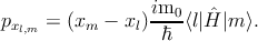
where Σ1 and Σ2 are the self-energies of the left/right contacts and Σs is the scattering self-energy. The self-energy due to electron-photon interaction is considered in this work. The Hamiltonian of the electron-photon interaction can be written as [160,161]:
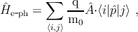 | (3.10) |
where  is the momentum operator and  is the vector potential. In second
quantization the vector potential is given by
is the momentum operator and  is the vector potential. In second
quantization the vector potential is given by
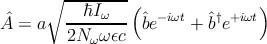 | (3.11) |
The direction of  is determined by the polarization of the field, which is denoted by the unit vector a.
As atomic orbitals in tight-binding are unknown, to evaluate the matrix elements
of the momentum, it is common to use the gradient approximation [162] where
the following commutator relation is used  =
=  [Ĥ,
[Ĥ, ].
].
Based on this approximation, for a transition from a state |m⟩ to a final state
|l⟩, the momentum matrix elements (pxl,m = ⟨l| x|m⟩) are
 | (3.12) |
The momentum matrix elements are therefore given by [163]
 | (3.13) |
Therefore, one can rewrite the electron-photon interaction Hamiltonian as:
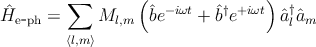 | (3.14) |
 | (3.15) |
where xm denotes the position of the carbon atom at site m and Nω is the photon population number with the frequency ω.
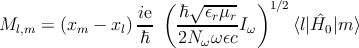
The photon flux (Iω), is defined as the number of photons per unit time per unit area [160,164]:
 | (3.16) |
where ϵr and μr are the relative dielectric and magnetic susceptibility,  is the
volume, and Pop is the incident power flux. The incident light is assumed to be
monochromatic with a power of Pop = 100kW∕cm2, and polarized along the
longitudinal axis, see Fig. 5.1.
is the
volume, and Pop is the incident power flux. The incident light is assumed to be
monochromatic with a power of Pop = 100kW∕cm2, and polarized along the
longitudinal axis, see Fig. 5.1.
We employed the lowest order self-energy of the electron-photon interaction based on the self-consistent Born approximation [165]:
![< ∑
Σ l,m(E ) = Ml,pMq,m
[ p,<q < ]
× N ωG p,q(E - ℏω ) + (N ω + 1)G p,q(E + ℏ ω)](diss87x.png) | (3.17) |
where the first term corresponds to the excitation of an electron by the absorption of a photon and the second term corresponds to the emission of a photon by de-excitation of an electron.