


Next: 3.4.2 Material Interfaces
Up: 3.4 Vacancy Sinks and
Previous: 3.4 Vacancy Sinks and
3.4.1 Grain Boundary Model
The grain boundary is modeled as a separate medium of width
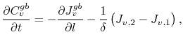
 embedded in a bulk, as depicted in Figure 3.3. Following the work of Fisher [149], the model takes into account two main mechanisms: vacancy diffusion along the grain boundary, which is considered a path of high diffusivity, and material exchange between the grain boundary and the grain bulk. Therefore, the vacancy dynamics inside the grain boundary can be described by
 |
(3.43) |
where  is the grain boundary vacancy concentration,
  is the vacancy flux along the grain boundary distance
  , and
, and
 are the fluxes from both sides of the grain boundary.
Figure 3.3:
Grain boundary model.
|
|
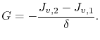
The last term in (3.43) connects the change in grain boundary vacancy concentration to the diffusing flux from/to the bulk. The difference
 corresponds to an actual loss/gain of vacancies, which is localized at the region representing the grain boundary. Thus, the vacancy generation/annihilation rate is given by
 |
(3.44) |
This loss/gain of vacancies can be described by a trapped vacancy concentration in the grain boundary, defined as  , in such a way that the generation/annihilation rate can be expressed as a function of the rate change of the trapped vacancy concentration as
 |
(3.45) |
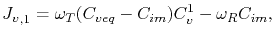
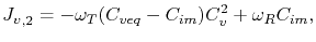
By treating the grain boundary as a region with the capability of absorbing or releasing vacancies, the fluxes in equation (3.44) can be expressed in terms of trapping and releasing events in a similar way to [150]. This yields [110]
 |
(3.46) |
 |
(3.47) |
where  is the trapping rate of vacancies,
  is the release rate,
 are the vacancy concentration in each grain section, and
  is the equilibrium vacancy concentration inside the grain boundary, given by
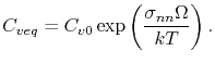 |
(3.48) |
 is the equilibrium vacancy concentration in the absence of stress and
 is the stress component normal to the grain boundary.
Substituting (3.46) and (3.47) in (3.44) and (3.45) one obtains
![$\displaystyle \G = \ensuremath{\ensuremath{\frac{\partial \Cim}{\partial t}}} =...
...s}\left\{\Ceq-\Cim\left[1+\frac{2\symOmR}{\symOmT(\CV^1+\CV^2)}\right]\right\}.$](img388.png) |
(3.49) |
For convenience, (3.49) is rewritten
![$\displaystyle \ensuremath{\ensuremath{\frac{\partial \Cim}{\partial t}}} = \fra...
...e}\left\{\Ceq-\Cim\left[1+\frac{2\symOmR}{\symOmT(\CV^1+\CV^2)}\right]\right\},$](img389.png) |
(3.50) |
with
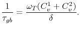 |
(3.51) |
 represents the characteristic time of a vacancy annihilation or generation process and it characterizes the efficiency of the grain boundary acting as a vacancy sink/source. The smaller the value of
, the more efficient is the source/sink mechanism and, according to (3.10), the faster the steady state condition for the vacancy concentration is reached.
represents the characteristic time of a vacancy annihilation or generation process and it characterizes the efficiency of the grain boundary acting as a vacancy sink/source. The smaller the value of
, the more efficient is the source/sink mechanism and, according to (3.10), the faster the steady state condition for the vacancy concentration is reached.
As in the numerical implementation the grain boundary is represented by the interface between two grains (
 ), the approximation
 can be used, so that (3.50) and (3.51) is further simplified to
![$\displaystyle \ensuremath{\ensuremath{\frac{\partial \Cim}{\partial t}}} = \fra...
...{\symGBRelTime}\left[\Ceq-\Cim\left(1+\frac{\symOmR}{\symOmT\CV}\right)\right],$](img394.png) |
(3.52) |
and
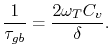 |
(3.53) |
Note that under the condition
 |
(3.54) |
equation (3.52) reduces to the Rosenberg-Ohring generation/annihilation function given in (2.21).
Next: 3.4.2 Material Interfaces
Up: 3.4 Vacancy Sinks and
Previous: 3.4 Vacancy Sinks and
R. L. de Orio: Electromigration Modeling and Simulation
![\includegraphics[width=0.80\linewidth]{chapter_electromigration_modeling/Figures/gbm.eps}](img379.png)