4.3.1 Newton's Method

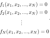
The non-linear system of equations, which results from the discretization described in Section 4.2, is solved in FEDOS using the conventional Newton method [153,154]. Generally, a non-linear system of $N$ equations is expressed as

$$\begin{aligned}&f_1(x_1, x_2, ..., x_N) = 0 \\ &f_2(x_1, x_2, .... ...\qquad\qquad\vdots \\ &f_N(x_1, x_2, ..., x_N) = 0 \end{aligned}.$$

If a given solution $x_j^{n-1}$, $j=1,...,N$, is known, these equations can expanded in the vicinity of $x_j^{n-1}$ using Taylor's series, which to the first order are approximated by

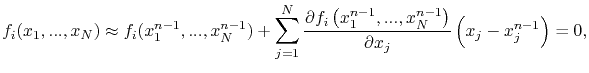$$f_i(x_1,...,x_N) \approx f_i(x_1^{n-1},...,x_N^{n-1})+\sum_{j=1}^... ..._N^{n-1}\right)}{\partial x_j}}\left(x_j - x_j^{n-1} \right) = 0,%\ i=1,...,N.$$ (4.69)

for $i=1,\dots,N$. The system of equations (4.69) is written in matrix form as

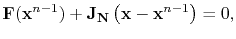$$\mathbf{F}(\mathbf{x}^{n-1}) + \mathbf{J_N}\left(\mathbf{x} - \mathbf{x}^{n-1} \right) = 0,$$ (4.70)

where $\mathbf{J_N}$ is the so-called Jacobian matrix, for which the entries are given by

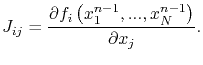$$J_{ij} = \ensuremath{\frac{\partial f_i\left(x_1^{n-1},...,x_N^{n-1}\right)}{\partial x_j}}.$$ (4.71)

Thus, the solution of (4.70) is

$$\mathbf{x}^n = \mathbf{x}^{n-1} - \mathbf{J_N}^{-1}\ \mathbf{F}(\mathbf{x}^{n-1}).$$ (4.72)

In FEDOS, instead of using (4.72), the linear system of equations

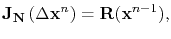$$\mathbf{J_N}\left(\Delta\mathbf{x}^n\right) = \mathbf R(\mathbf{x}^{n-1}),$$ (4.73)

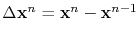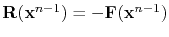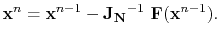
is assembled and solved, so that the increments $\Delta\mathbf{x}^n = \mathbf{x}^n - \mathbf{x}^{n-1}$ are determined. Here, $\mathbf R(\mathbf{x}^{n-1})=-\mathbf{F}(\mathbf{x}^{n-1})$ is called residual. In this way, the new approximate solution $\mathbf{x}^n$ is updated according to

$$\mathbf{x}^n = \mathbf{x}^{n-1} + \Delta\mathbf{x}^n.$$ (4.74)

These calculations are performed as an iterative process, where the solution of the $n-1$ iteration is used to compute the new solution. The accuracy of the new approximate solution is controlled by the conditions

$$\Vert\mathbf{x}^n - \mathbf{x}^{n-1}\Vert \leq \epsilon_{er},$$ (4.75)

where $\epsilon_{er}$ is a given tolerance for the solution error, and

$$\Vert\mathbf R(\mathbf{x}^n)\Vert \leq \epsilon_{res},$$ (4.76)

where $\epsilon_{res}$ is a given tolerance for the residual and $\Vert\cdot\Vert$ represents the Euclidean norm. The iterative procedure is terminated, if both criteria are fulfilled.