4.3.2 Assembly of the Electro-Thermal Problem

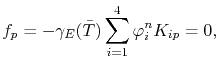
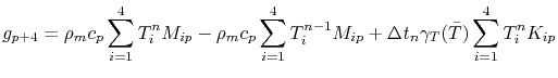
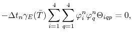
The discretization of the electrical and the thermal problem, (4.32) and (4.40), respectively, forms a non-linear system of equations for a tetrahedral element given by

$$\begin{aligned}&\mathbf{F}(\boldsymbol\symElecPot, \boldsymbol\... ...athbf{G}(\boldsymbol\symElecPot, \boldsymbol\T) = 0 \end{aligned}$$

where $\mathbf{F}(\boldsymbol\symElecPot, \boldsymbol\T)$ corresponds to

$$f_p = -\symElecCond(\bar\T)\ensuremath{\sum_{i=1}^{4}{\symElecPot_i^n}}K_{ip} = 0,$$ (4.78)

and $\mathbf{G}(\boldsymbol\symElecPot, \boldsymbol\T)$ to

$$g_{p+4} = \symMatDens\symSpecHeat \sum_{i=1}^{4}\T_i^n M_{ip} - \... ...T_i^{n-1} M_{ip} + \Delta t_n \symThermCond(\bar\T) \sum_{i=1}^{4}\T_i^n K_{ip}$$

$$- \Delta t_n \symElecCond(\bar\T) \sum_{i=1}^4\sum_{q=1}^4 \symElecPot_i^n\symElecPot_q^n \Theta_{iqp} = 0,$$ (4.79)

for $p=1,\dots,4$.

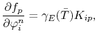
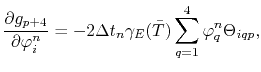
Applying Newton's method, the element Jacobian matrix for the electro-thermal problem has the form

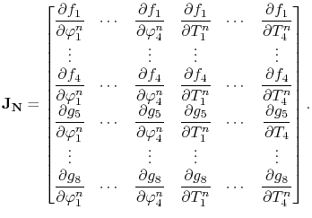
$$\mathbf{J_N} = \begin{bmatrix}\displaystyle\ensuremath{\frac{\par... ... &\displaystyle\ensuremath{\frac{\partial g_8}{\partial \T_4^n}} \end{bmatrix}.$$ (4.80)

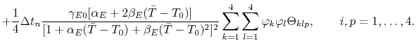
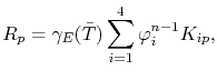
Since the global system for the electro-thermal problem is constructed following the assembly procedure described in Section 4.1.2, the Jacobian matrix is the nucleus matrix to be computed for each element of the mesh. The matrix entries for the electrical equation (4.78) are given, in general, by

$$\ensuremath{\frac{\partial f_p}{\partial \symElecPot_i^n}} = \symElecCond(\bar\T) K_{ip},$$ (4.81)

$$\ensuremath{\frac{\partial f_p}{\partial \T_i^n}} = -\ensuremath{... ...T-\TO)+\symQuadTempCoef_E(\bar\T-\TO)^2]^2}\sum_{k=1}^4 \symElecPot_k^n K_{kp},$$ (4.82)

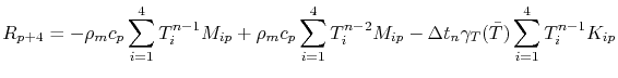
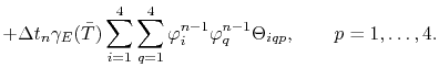
and the entries for the thermal equation (4.79) are computed by

$$\ensuremath{\frac{\partial g_{p+4}}{\partial \symElecPot_i^n}} = -2\Delta t_n \symElecCond(\bar\T) \sum_{q=1}^4 \symElecPot_q^n\Theta_{iqp},$$ (4.83)

$$\ensuremath{\frac{\partial g_{p+4}}{\partial \T_i^n}} = \symMatDe... ...f_T(\bar\T-\TO)+\symQuadTempCoef_T(\bar\T-\TO)^2]^2} \sum_{k=1}^4 \T_k^n K_{kp}$$

$$+ \frac{1}{4}\Delta t_n \frac{\gamma_{E0}[\symLinTempCoef_E+2\sym... ...1}^4\sum_{l=1}^4 \symElecPot_k\symElecPot_l\Theta_{klp},\qquad i,p = 1,\dots,4.$$ (4.84)

The right-hand side of the linear system (4.73) is assembled by the residuals

$$R_p = \symElecCond(\bar\T)\ensuremath{\sum_{i=1}^{4}{\symElecPot_i^{n-1}}}K_{ip},$$ (4.85)

$$R_{p+4} = -\symMatDens\symSpecHeat \sum_{i=1}^{4}\T_i^{n-1} M_{ip... ...{n-2} M_{ip} - \Delta t_n \symThermCond(\bar\T) \sum_{i=1}^{4}\T_i^{n-1} K_{ip}$$

$$+ \Delta t_n \symElecCond(\bar\T) \sum_{i=1}^4\sum_{q=1}^4 \symElecPot_i^{n-1}\symElecPot_q^{n-1} \Theta_{iqp}, \qquad p = 1,\dots,4.$$ (4.86)