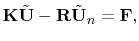
4.4 FEM solution for the two-dimensional Helmholtz equation
Finite element methods (FEM), initially developed for structural mechanics
[70], are widely used for numerical simulations of electromagnetic fields
[15], [23], [71], [72],
[73]. Some advantages of the finite element method are listed below.
- A sparse system matrix enables the simulation of problems with a large
number of unknowns.
- Suitable for inhomogeneous simulation domains.
- Adaptability to arbitrary geometries by triangular meshes for
two-dimensional
simulations and tetrahedral meshes for three-dimensional
problems.
- Suitable for inhomogeneous simulation domains.
- Existence of an unambiguous solution for elliptical partial differential
equations.
This means convergence of the solution error towards zero with mesh
refinement.
The finite element method provides an approximate solution  for the elliptical
partial differential equation (4.13). The residuum (approximation
error) of this solution is
for the elliptical
partial differential equation (4.13). The residuum (approximation
error) of this solution is
 |
(4.24) |
For consistence to the voltage and current directions, defined by the impedance matrix
in (4.17), a negative sign has been used for the current density
 , as opposed to the sign in (4.13). The residuum
  ,
weighted with a function
,
weighted with a function  , will vanish on average over the simulation domain. This
is expressed in the variation integral
, will vanish on average over the simulation domain. This
is expressed in the variation integral
 |
(4.25) |
 denotes the whole simulation domain, that is, the parallel plane surface.
Applying Green's theorem, (4.25) is transformed to the weak
formulation
denotes the whole simulation domain, that is, the parallel plane surface.
Applying Green's theorem, (4.25) is transformed to the weak
formulation
 |
(4.26) |
 is the boundary curve of the parallel plane surface
,
is the boundary curve of the parallel plane surface
,
 is the line segment of this boundary curve and
 is the normal derivation of at the boundary.
is expressed by
is the normal derivation of at the boundary.
is expressed by
 |
(4.27) |
Where
 denote the finite element base functions,
 are the
values of the solution at the mesh points, and
are the
values of the solution at the mesh points, and  denotes the number of mesh nodes.
According to the method of Galerkin, the weighting function is
denotes the number of mesh nodes.
According to the method of Galerkin, the weighting function is
 |
(4.28) |
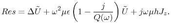
Linear base functions on a triangular mesh are selected for the finite element
discretization. Barycentric coordinates are utilized according to
Figure 4.5.
![\includegraphics[width=7cm,viewport=185 590 390 735,clip]{{pics/Barycentric.eps}}](img301.png)
Figure 4.5:
Barycentric (triangular) coordinates  and
and  . Coordinates
(,) become (1,0), (0,1), and (0,0) in the nodes 1, 2, and 3,
respectively.
. Coordinates
(,) become (1,0), (0,1), and (0,0) in the nodes 1, 2, and 3,
respectively.
With this coordinate system definition the base functions are
 and and 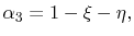 |
(4.29) |
with indexes according to the triangle node numbers in Figure 4.5.
The relation of the barycentric to the cartesian coordinates of the triangular nodes is
 |
(4.30) |
with
 |
(4.31) |
 is the surface area of the triangle with index
  . With
equations (4.27) and (4.28), (4.26)
becomes the linear equation system
. With
equations (4.27) and (4.28), (4.26)
becomes the linear equation system
 |
(4.32) |
for the voltages
 on the mesh nodes.
 denotes
the vector of the normal derivatives of
at the boundary. At open
boundaries the PMC boundary condition requires vanishing
. On
closed metallic edges a Dirichlet boundary has to be introduced, by setting the boundary
node voltage to zero and reducing the order of the linear system accordingly. Since the
weighting function is set to zero in the boundary nodes with Dirichlet condition, the
term with
vanishes also at Dirichlet boundaries
and (4.32) is reduced to
denotes
the vector of the normal derivatives of
at the boundary. At open
boundaries the PMC boundary condition requires vanishing
. On
closed metallic edges a Dirichlet boundary has to be introduced, by setting the boundary
node voltage to zero and reducing the order of the linear system accordingly. Since the
weighting function is set to zero in the boundary nodes with Dirichlet condition, the
term with
vanishes also at Dirichlet boundaries
and (4.32) is reduced to
 |
(4.33) |
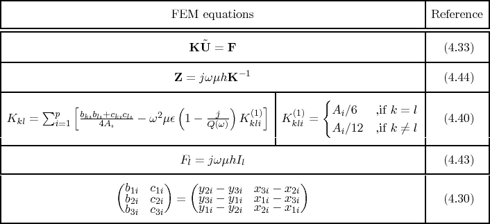
The system matrix elements  are obtained from the solution of
![$\displaystyle K_{kl}=\int_{\mathcal{A}}\left[\vec{\nabla}\alpha_{k}\cdot\vec{\n...
...1-\frac{j}{Q(\omega)}\right)\alpha_{k}\alpha_{l}
\right]\textrm{d}\mathcal{A}.$](img308.png) |
(4.34) |
The term
 in( 4.34)
becomes
in( 4.34)
becomes
 |
(4.35) |
With the base functions
 and and  |
(4.36) |
and (4.30), the partial derivatives of (4.35) become
 |
(4.37) |
Using these partial derivatives expressions (4.34) becomes
![$\displaystyle K_{kl}=\int_{\mathcal{A}}\left[\frac{b_{ki}b_{li}+c_{ki}c_{li}}{4...
...epsilon\left(1-\frac{j}{Q(\omega)}\right)\xi\eta
\right]\textrm{d}\mathcal{A}.$](img314.png) |
(4.38) |
Utilizing
 |
(4.39) |
from [23], the integral of (4.38) is solved analytically
and the coefficients of the FEM matrix finally become
![$\displaystyle K_{kl}=\sum_{i=1}^{p}\left[\frac{b_{ki}b_{li}+c_{ki}c_{li}}{4A_{i}}
-\omega^{2}\mu\epsilon\left(1-\frac{j}{Q(\omega)}\right)K_{kli}^{(1)}\right]$](img316.png) |
(4.40) |
with
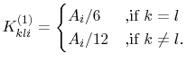 |
(4.41) |
At the node position
 the port excitation current is
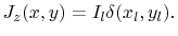 |
(4.42) |
 is the Dirac pulse function and
  is the node index running from
one to the number of nodes . With (4.26), (4.28), (4.36), and (4.42), the
coefficients of the excitation vector
is the node index running from
one to the number of nodes . With (4.26), (4.28), (4.36), and (4.42), the
coefficients of the excitation vector
 in (4.33) become
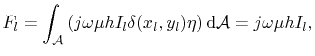 |
(4.43) |
because the weighting function is unity at node position
according
to the base function definition in (4.29). With this port current
excitation definition the impedance matrix, which relates the voltages on the mesh nodes
to the node excitation currents, is
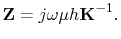 |
(4.44) |
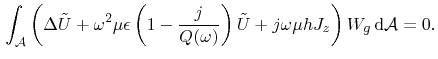
Figure 4.6 depicts a comparison of the analytic results
from (4.18) to the FEM results for the impedance  of a
port at position
of a
port at position
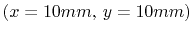 on a rectangular cavity with dimensions
  ,
,
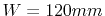 and
and  . Although this FEM simulation was carried out using a very coarse
mesh with
. Although this FEM simulation was carried out using a very coarse
mesh with
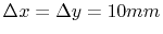 , the results of this simulation match the analytical
solution well. Thus, the proposed FEM method provides an efficient and accurate solution
for arbitrarily shaped parallel plane cavities. In the case of a large number of
excitation ports, the FEM method is even more efficient than the analytical solution.
While the analytical method requires the calculation of the double sum term
in (4.18) for each coefficient in the port impedance
matrix (4.17), the FEM solution requires only one inversion of the
sparse system matrix
, the results of this simulation match the analytical
solution well. Thus, the proposed FEM method provides an efficient and accurate solution
for arbitrarily shaped parallel plane cavities. In the case of a large number of
excitation ports, the FEM method is even more efficient than the analytical solution.
While the analytical method requires the calculation of the double sum term
in (4.18) for each coefficient in the port impedance
matrix (4.17), the FEM solution requires only one inversion of the
sparse system matrix
 . Linear base functions and a triangular mesh enable an
efficient, analytical composition of the system matrix
and the excitation
vector
with (4.40) and (4.43) respectively.
Since a high accuracy is achieved with the linear base functions even on a coarse mesh,
there is no need for higher order base functions. Table 4.2 contains
a summary of the FEM equations.
. Linear base functions and a triangular mesh enable an
efficient, analytical composition of the system matrix
and the excitation
vector
with (4.40) and (4.43) respectively.
Since a high accuracy is achieved with the linear base functions even on a coarse mesh,
there is no need for higher order base functions. Table 4.2 contains
a summary of the FEM equations.
![\includegraphics[height=6.3 cm,viewport=180 285 420
500,clip]{pics/MagAnalyticFEM.eps}](img323.png)
![\includegraphics[height=6.3 cm,viewport=180 285 415
500,clip]{pics/PhAnalyticFEM.eps}](img324.png)
| (a) Magnitude comparison. | (b) Phase angle comparison. |
Figure 4.6:
Comparison of between the analytical
solution (4.18) and the FEM solution. Cavity dimensions are
(, , ), the position of the port for the is
and the mesh spacing is
.
In the following the FEM equations are summarized.
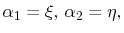
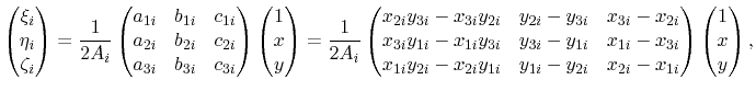
Table 4.2:
Summary of the FEM equations.
 |
C. Poschalko: The Simulation of Emission from Printed Circuit Boards under a Metallic Cover