5.3 Validation of the trace introduction by HFSS® simulations
An empirical validation of the proposed trace introduction method
with (5.6) and (5.9) is carried out by
HFSS® simulations. HFSS® is a FEM based
three-dimensional full wave simulation tool from Ansoft®
[76].
A first HFSS® enclosure model with a trace, depicted in
Figure 5.5(c), is simulated with ports at the source and the load positions
of the trace and three measurement ports at the slot. In a second HFSS®
model, presented in Figure 5.5(d), the trace is removed and ports are
defined between the bottom and the cover plane of the enclosure in the same positions as
the trace load and source ports in the first model. The enclosure cover has been removed
in Figure 5.5(c) and Figure 5.5(d) to enable a view of the
inside. The enclosure with cover is depicted in Figure 5.5(b), and
Figure 5.5(a) depicts the bounding box, with absorbing boundaries at
the surface, that surrounds the enclosure in the simulation models.
Lumped ports are defined in HFSS® on rectangular surfaces which are
small compared to the wavelength of the highest simulated frequency.
HFSS® calculates the S-parameter matrix of the ports, which is
transformed to a Z-parameter matrix. Proven convergence of the HFSS®
simulation is given through a monotone decrease of S-parameter results differences from
two consecutive adaptive mesh refinement iterations. For the model in
Figure 5.5(c) the transfer impedance from the trace source port to a
measurement port at the slot is
 |
(5.10) |
where
 ,
,
 and
and
 are the Z-parameters of this
HFSS® model and
are the Z-parameters of this
HFSS® model and  is an arbitrary trace load.
HFSS® would also enable the trace load in the model to be defined and
the transfer impedance to, thus, be obtained directly instead of
using (5.10). However, this would require one HFSS®
simulation for each load. Therefore, results for different loads are obtained efficiently
by the described model which requires only one HFSS® simulation.
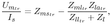
According to the described trace introduction method, the transfer impedance is also
obtained with (5.6) and (5.9) and the
Z-matrix (4.17) of the HFSS® model in
Figure 5.5(d). The characteristic impedance of the trace
in (5.6) is calculated in accordance with [77]
is an arbitrary trace load.
HFSS® would also enable the trace load in the model to be defined and
the transfer impedance to, thus, be obtained directly instead of
using (5.10). However, this would require one HFSS®
simulation for each load. Therefore, results for different loads are obtained efficiently
by the described model which requires only one HFSS® simulation.
According to the described trace introduction method, the transfer impedance is also
obtained with (5.6) and (5.9) and the
Z-matrix (4.17) of the HFSS® model in
Figure 5.5(d). The characteristic impedance of the trace
in (5.6) is calculated in accordance with [77]
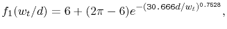
![$\displaystyle Z_{w}=(60\Omega)\ln\left[\frac{f_{1}(w_{t}/d)}{w_{t}/d}+\sqrt{1+\left(\frac{2d}{w_{t}}\right)^2}\right],$](img355.png) |
(5.11) |
and
 |
(5.12) |
where  is the trace width and
  is the trace height above the ground plane.
Equation (5.11) with the adjustment function
(5.12) approximates the exact conformal mapping solution from
[78], [79], for the characteristic impedance of a
thin sheet trace in air. The approximation uncertainty is below 0.03% for
is the trace height above the ground plane.
Equation (5.11) with the adjustment function
(5.12) approximates the exact conformal mapping solution from
[78], [79], for the characteristic impedance of a
thin sheet trace in air. The approximation uncertainty is below 0.03% for
 1000.
1000.
For the purpose of simulating traces on a real PCB, the dielectric material of the PCB
has to be considered with appropriate formulations [77],
[80].
A comparison of the transfer impedances from both models validates the trace introduction
method without any further simplifications, as there would be, if the cavity model were
to be used instead of HFSS® simulation. For instance, the radiation
from the open enclosure slot is considered by surrounding the enclosure with the boundary
box in the HFSS® model (Figure 5.5(a)).
![\includegraphics[height=4 cm,viewport=100 475 505 735
,clip]{pics/Encl_cover_box.eps}](img359.png)
![\includegraphics[height=3.4 cm,viewport=72 520 527 730
,clip]{pics/Encl_cover.eps}](img360.png)
| (a) Enclosure model inside a bounding box. | (b) Enclosure model with cover. |
![\includegraphics[height=3.8 cm,viewport=70 500 525 720
,clip]{pics/Encl_trace.eps}](img361.png)
![\includegraphics[height=3 cm,viewport=80 535 505 710
,clip]{pics/Encl_ports.eps}](img362.png)
| (c) Model with a trace (cover removed). | (d) Model with ports (cover removed). |
Figure 5.5:
HFSS® models for the validation of the trace introduction
method.
Figure 5.6 depicts the results of the described transfer
impedance comparison for a trace at position (x=67mm, y=50mm), the measurement port at
position (x=67mm, y=104mm) and trace loads of 0 Ohm, 1e9 Ohm, and 50 Ohm. The trace
length is l=5mm, the trace width is =2mm, the trace height above ground is
d=0.65mm, and the enclosure dimensions are (L=134mm, W=104mm, h=7mm). To cover the whole
ground-plane area, comparisons from nine trace positions are collected in
Appendix A.1.
![\includegraphics[height=6.5 cm,viewport=180 285 420 500,clip]{pics/cZ/M1_6_1.eps}](img363.png)
![\includegraphics[height=6.5 cm,viewport=180 285 415 500,clip]{pics/cZ/A1_6_1.eps}](img364.png)
| Load: 0 Ohm, magnitude. | Load: 0 Ohm, phase angle. |
![\includegraphics[height=6.5 cm,viewport=180 285 420 500,clip]{pics/cZ/M1_6_2.eps}](img365.png)
![\includegraphics[height=6.5 cm,viewport=180 285 420 500,clip]{pics/cZ/A1_6_2.eps}](img366.png)
| Load: 1e9 Ohm, magnitude. | Load: 1e9 Ohm, phase angle. |
![\includegraphics[height=6.5 cm,viewport=180 285 420 500,clip]{pics/cZ/M1_6_3.eps}](img367.png)
![\includegraphics[height=6.5 cm,viewport=180 285 420 500,clip]{pics/cZ/A1_6_3.eps}](img368.png)
| Load: 50 Ohm, magnitude. | Load: 50 Ohm, phase angle. |
Figure 5.6:
Transfer impedance from the trace source current to the slot measurement port at (67mm,104mm). The trace is located at position (67mm,50mm) and the trace length is 5mm. Trace orientation in y-direction. Comparison of HFSS results from a model with a trace and the results obtained with (5.6), (5.9) and a HFSS model with ports.
More comparisons are presented for a variation of the enclosure height, for a variation
of the trace height above the ground plane, and for parallel planes with four open edges
in Appendix A.2. All comparisons show very good
agreement, both in magnitude and phase. Thus, the proposed trace introduction method with
the analytical coupling factor is generally sufficient for electromagnetic emission
simulation.
C. Poschalko: The Simulation of Emission from Printed Circuit Boards under a Metallic Cover