|
|
|
|
Previous: F.1 Electron-Electron Interaction Up: F.1 Electron-Electron Interaction Next: F.2 Electron-Phonon Interaction |
|
|
|
|
Previous: F.1 Electron-Electron Interaction Up: F.1 Electron-Electron Interaction Next: F.2 Electron-Phonon Interaction |
 |
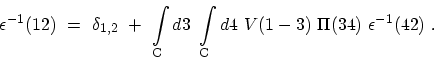
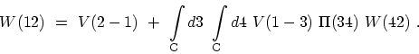
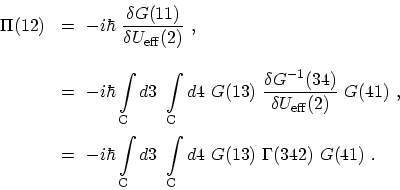
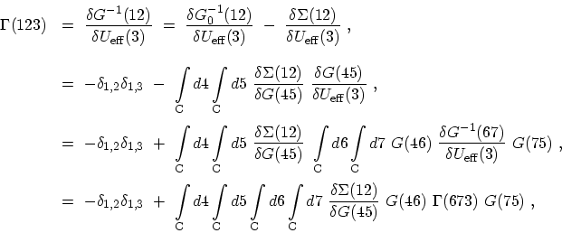
(F.13) |