2.4.1 Electronic Band Structure of Graphene

Within the tight-binding method the two-dimensional energy dispersion relations of graphene can be calculated by solving the eigen-value problem for a HAMILTONian $H_\mathrm{g-2D}$ associated with the two carbon atoms in the graphene unit cell [12]. In the SLATER-KOSTER scheme one gets^2.1

$$H_\mathrm{g-2D} \ = \ \left[ \begin{array}{cc} 0 & f(k)\\ - f^\dagger(k) & 0 \end{array} \right] \ .$$ (2.3)

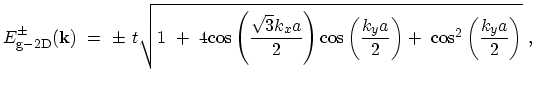
where $f(k)=- t(1+e^{i{\bf k}\cdot.{\bf a_1}}+e^{i{\bf k}\cdot{\bf a_2}})= -t(1+2e^{\sqrt{3}k_xa/2}\mathrm{cos}(k_ya/2))$ and $t$ is the nearest neighbor C-C tight binding overlap energy^2.2 [29]. Solution of the secular equation $\mathrm{det}(H_\mathrm{g-2D}-EI)=0$ leads to

$$E_\mathrm{g-2D}^{\pm}({\bf k}) \ = \ \pm \ t\sqrt{1 \ + \ 4\mathr... ...\left(\frac{k_ya}{2}\right) + \ \mathrm{cos}^2\left(\frac{k_ya}{2}\right) } \ ,$$ (2.4)

where the $E_\mathrm{g-2D}^+$ and $E_\mathrm{g-2D}^-$ correspond to the $\pi ^*$ and the $\pi$ energy bands, respectively. Figure 2.6 shows the electronic energy dispersion relations for graphene as a function of the two-dimensional wave-vector ${\bf k}$ in the hexagonal BRILLOUIN zone.

Figure 2.6: The energy dispersion relations for graphene are shown through the whole region of the BRILLOUIN zone. The lower and the upper surfaces denote the valence $\pi$ and the conduction $\pi ^*$ energy bands, respectively. The coordinates of high symmetry points are $\Gamma =(0,0)$, $\mathrm{K}=(0,2\pi/3a)$, and $\mathrm{M}=(2\pi/\sqrt{3}a,0)$. The energy values at the $\mathrm{K}$, $\mathrm{M}$, and $\Gamma$ points are 0, $t$, and $3t$, respectively.

M. Pourfath: Numerical Study of Quantum Transport in Carbon Nanotube-Based Transistors