7.3 Rotational Symmetries

Algorithm 5.6 and Algorithm 5.7 are used to generate the templated meshes for objects with rotational symmetries. The implementation first creates a line mesh of the geometry using the requested cell size. For 2D objects, the Triangle software is used to generate a volumetric triangle mesh using the line mesh as a surface mesh. The surface mesh is not altered. For 3D objects, Triangle is used to generate triangle surfaces with triangle sizes suitable for the desired volumetric cell size. These triangle surfaces are used to generate the template surface meshes based on the boundary patch partition. For each template a volumetric mesh is generated using Tetgen without inserting Steiner points on any surface mesh.

Two cases with rotational symmetries are investigated:

(i)

A 2D $n$-polygon (Figure 7.5a)

(ii)

A 3D open through-silicon via (TSV) structure [28] (Figure 7.5f)

Figure 7.5: Benchmark objects with rotational symmetries

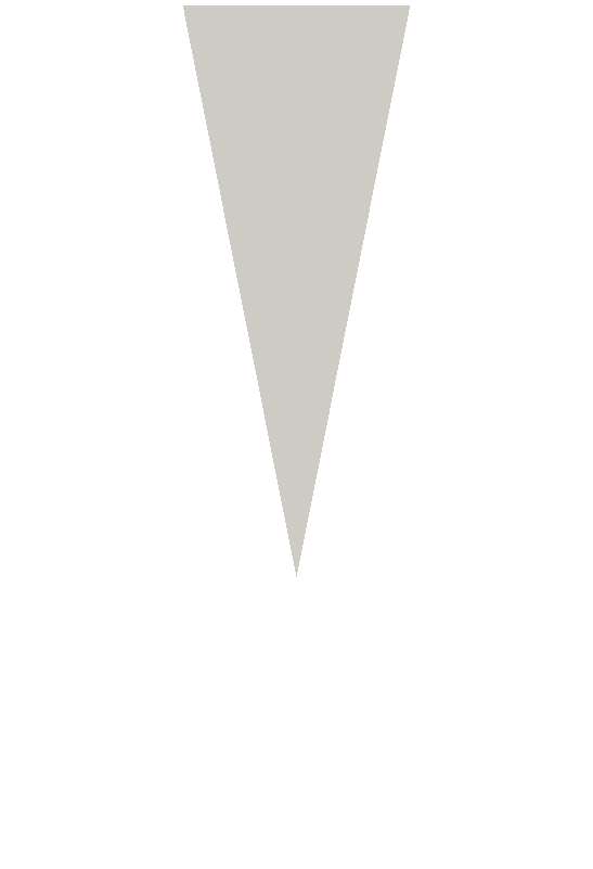
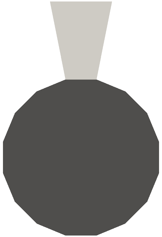
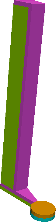
Both objects have a rotational symmetry order of $16$. On the left, the object geometry is visualized. In the middle, templates for the classical templated approach with one slice are shown. On the right, the small angle optimization (SAO) templates are given with one slice and the middle part which is a regular $16$-polygon or regular $16$-prism. The templates are visualized in different colors.

The objects visualized in Figure 7.5 have been synthetically generated. While the first one (the $n$-polygon) is merely used for a proof-of-concept, the open TSV structure represents an object used in microelectronic applications. Geometries with rotational symmetry orders of $8, 16, 32, 64$, and $128$ have been generated for both objects. The concepts presented in Section 6.3 (in this section referred to as slice template or ST) have been applied to all rotationally symmetric objects. Additionally, the small angle optimization (SAO) approach (cf. Section 6.3.2) has also been used in the benchmarks. Therefore, the conventional mesh generation has been benchmarked against a templated version with and without small angle optimization.

Benchmark results for the 2D $n$-polygon are given in Figure 7.6. The results are similar to the ones from the previous section: The expected savings in runtime and memory usage are achieved for meshes with a high number of cells. The runtime speedups are larger than a factor of one for cell counts larger than $10^3$ and larger than a factor of five for cell counts larger than $5 \times 10^4$. The behavior of the memory savings is more stable. Memory savings larger than one are achieved for almost all benchmarks. Memory savings larger than a factor of five are obtained for both approaches (ST and SAO) for cell counts larger than $5 \times 10^3$ using the data structure without SVB. The data structure with SVB performs worse. However, memory savings larger than a factor of ten are achieved for large cell count values. The runtime speedups scale well with the rotational symmetry order for cell counts larger than $10^5$ (cf. Figure 7.6e). Memory savings also scale well with the rotational symmetry order for meshes with more than $5 \times 10^3$ cells (cf. Figure 7.6f). However, memory savings with SVB (visualized using $\circ$) are smaller. For high rotational symmetry orders, the memory savings using a data structure with SVB even starts to decrease (cf. Figure 7.6f) due to the large number of vertices on instance interfaces which increase the bookkeeping effort.

Figure 7.6: Benchmark results for the 2D $n$-polygon

The top row and middle row visualizes benchmark results for different cell count values for the TS and SAO approach, respectively. The dashed black lines indicate the expected runtime and memory savings of the different rotational symmetry orders $8, 16, 32, 64$, and $128$. Benchmark results for different rotational symmetry orders are visualized in the bottom row. Only meshes with a minimal cell count of $10^5$ are considered for the rotational symmetry plots.

Figure 7.7: Smallest angle quality histograms for $n$-polygon benchmarks

A selection of smallest angle quality histograms of meshes of $n$-polygons. The histogram bins are given in log scale for better visualization of the bad quality bins. The quality histograms of the conventionally generated meshes are visualized in the left column. The quality histogram of the structure instance of the TS is given in the middle column. The right column shows quality histograms of the SAO approach. Bins colored in red indicate cells with quality worse than the configured value. The smallest angle quality value constraint is visualized using the black vertical line. The smallest angle of the TS approach structure instance of every presented benchmark does not fulfill the configured values as indicated by the red histogram bins. Additionally, the mesh quality of the structure instances of the SAO approach is even better then the quality of the corresponding conventionally generated mesh as indicated by a slightly higher dominance of larger smallest angles in the quality histograms of the SAO approach.

Figure 7.8: Quality comparison of meshes generated for a $16$-polygon

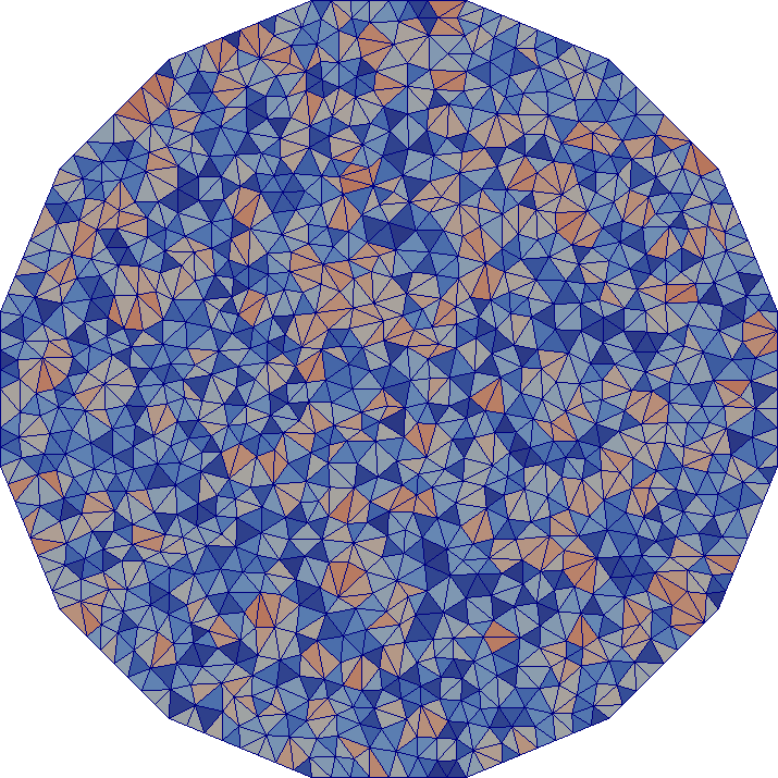
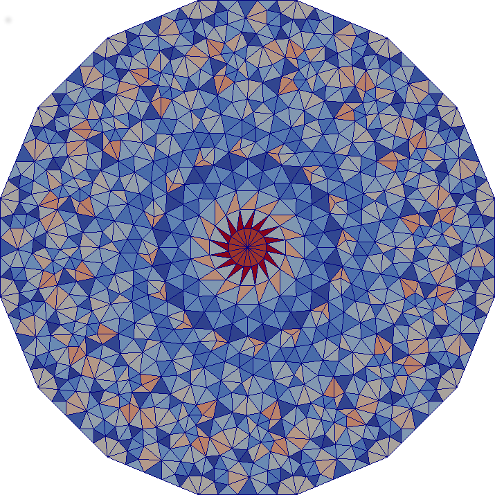
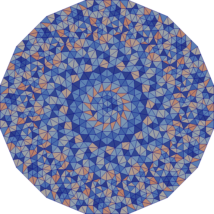
All meshes have been generated with a requested cell size of $2.5 \times 10^{-3}$ and a smallest angle of $30\degree$. Elements near the center of (top right picture) have a smallest angle which violates the smallest angle constraint. The conventionally generated mesh (top left picture) and the SAO approach (bottom left picture) both fulfill the requested element quality.

The smallest angle quality parameters $10\degree, 20\degree$, and $30\degree$ are used for the rotational symmetry benchmarks. While the conventional mesh generation algorithm was always able to fulfill the desired quality parameters, the TS approach has issues due to small angles near the center of rotation for high rotational symmetry orders (cf. Section 6.3.2). However, the SAO approach was able to generate meshes with smallest element angles larger than the configured values. A selection of quality histograms is given in Figure 7.7, example meshes of a selected benchmark are visualized in Figure 7.8.

Benchmark results for the 3D open TSV structure are given in Figure 7.9. Runtime speedups from $5$ up to $100$ can be achieved. However, no correlation to the cell counts of the meshes is observed for the 3D structure. Memory savings without SVB ranging from $10$ to $100$ are observed (cf. Figure 7.9b). However, with SVB, the memory savings are much smaller ranging from a factor of two to a factor of ten. Similar to the runtime speedup behavior, the memory savings are not correlated to the cell counts. The memory savings, however, are slightly better as depicted by Figure 7.9d. The runtime speedups also scale well with the rotational symmetry order of the object (cf. Figure 7.9e). This is also true for the memory savings when using the data structure without SVB. The behavior when using the data structure with SVB, however, is completely different (cf. Figure 7.9f). The memory savings start to decrease for high rotational symmetry orders. This behavior can be explained by the high vertex count on the instance interfaces for high rotational symmetry orders. A high number of vertices on instance interfaces increases the memory usage of the shared vertex bookkeeping in turn resulting in reduced memory savings.

Figure 7.9: Benchmark results for the 3D open TSV structure

The top row and middle row visualizes benchmark results for different cell count values for the template slice and small angle optimization approach, respectively. The dashed black lines indicate the expected runtime speedups and memory savings of the different rotational symmetry orders $8, 16, 32, 64$, and $128$. Benchmark results for different rotational symmetry orders are visualized in the bottom row. Only meshes with a minimal cell count of $10^5$ are considered for the rotational symmetry plots.